

INTRODUCTION
The first experiments of nuclear magnetic resonance (NMR) were performed in 1946 and since then its application in physics, chemistry, and biology has been phenomenal. Magnetic resonance (MR) is a technique for probing atoms and molecules based upon their interaction with an external magnetic field (B0). Initially NMR was used for chemical structure elucidation, and its potential related to medicine was recognized almost at the same time. The most familiar application of NMR phenomenon to the common man and the clinical community is magnetic resonance imaging (MRI), which is used to produce anatomic images for diagnostic purposes of various pathologies. In 1973, high-resolution phosphorus (31P) NMR studies of intact blood cells1 and later on muscle tissues were reported2, 3. Ackerman et al4 reported 31P NMR study of skeletal muscle and brain metabolism noninvasively in small animals using a surface coil. With the availability of larger magnets extension to human 31P MR studies, followed later.
In 1971, Damadian5 reported that the NMR relaxation time constants (T1 and T2) are different for normal and malignant tissues and could have diagnostic value, which formed the basis of development of MRI. Lauterbur in 1973 produced the first image of a live animal6. Later MR images of human organs such as finger7, hand8, and wrist9 were reported. With the development of long-hold magnets with high homogeneity, strong magnetic field gradients, RF electronics, and powerful computers, the whole body MRI systems became a reality for many clinical applications. Today MR is experiencing a rapid expansion and has achieved amazing level of success as an important tool to study several disease processes in clinical and experimental research. This is due to its noninvasive nature, avoidance of ionizing radiation and its ability to generate high-resolution images. MRI produces spatial display of the distribution of nuclei (such as hydrogens) and provides high-resolution morphological picture (anatomical information) with superior contrast resolution compared to other currently available imaging modalities. Moreover, MR images can be obtained in transverse, sagittal, coronal and oblique planes without moving the object/subject. Being 2noninvasive, the method can be used for repetitive measurements, which is useful to study the pharmacokinetics and efficacy of drugs. These features have made MRI as one of the most useful soft tissue diagnostic modality for many neurological, cardiac, musculoskeletal and other pathologies10–12.
The other important application of NMR phenomenon in clinical medicine is NMR spectroscopic investigation of living systems termed as in vivo MR spectroscopy (MRS). The technique of in vivo MRS can also be used as a unique means to probe the biochemistry of living systems with diagnostic importance. In vivo MRS of cells and of organs and tissues in humans and animals, are an extension of high-resolution NMR used for studying structure of molecules, but applied to more complex systems. It can be used to observe different metabolites present in a particular region of tissues and organs. The determination of the concentration and relative levels of these metabolites provide information on normal and diseased tissues. MRI and in vivo MRS, both are based on the same physical phenomenon as NMR and the principles are well described in many textbooks10–16. The significant technical difference between MRI and MRS is that in MRI the signal is acquired in the presence of magnetic field gradients while for MRS it is prerequisite to have a homogeneous magnetic field to observe the chemical shift differences of metabolites and, therefore, no magnetic field gradients are applied during signal acquisition. MRI and in vivo MRS have evolved more or less independently, however, most in vivo localized MRS use MR images to guide the region of interest (ROI) or volume of interest (VOI) for spectroscopic investigations. Thus the success of MRI had considerable impact in the development of in vivo MRS methodologies which can be used to detect and estimate the concentration of different metabolites present in a particular region of the tissue or organ. The relative level of these metabolites provide information on the status of normal and pathological tissues. Like MRI, MRS can also be used repetitively to monitor the response of tumors to various therapeutic modalities, efficacy of drugs and to understand the different metabolic processes11, 14–16.
This chapter presents the basic concepts of MRI and in vivo MRS in qualitative terms without the use of quantum physics. It is beyond the scope of this article to present a comprehensive review of the theory and the various applications of MRI and MRS, however, the organization and content presented would form the basis to follow the various applications of MRI and MRS described later in this volume.
CONCEPTS
Theory
NMR is the magnetic interaction between nuclei of atoms and radio-frequency (RF) field (B1) in the presence of an external magnetic field (B0). According to quantum mechanics, a subatomic particle such as proton has quantized angular momentum, called spin (I). Associated with spin is a magnetic moment. Hydrogen atom has only one proton as nucleus and hence this property can be observed by looking at hydrogen. The human body consists mostly of water and fat and since hydrogen is a constituent atom in water and fat, we have a potential medical application. Since each water molecule has two associated hydrogen atoms covalently bound to an oxygen atom, there are approximately 5 × 1027 hydrogen nuclei in an adult human body.


Fig. 1.1: (A) Spin orientation in human tissue sample in the absence of external magnetic field (Bo). (B) In the presence of an external magnetic field the spins orient themselves along the magnetic field direction (z-axis) with some spins in the parallel and some anti-parallel state with respect to the magnetic field. Transition between the energy levels is possible by the application of RF energy (equivalent to ∆E) applied at the resonant frequency (ν0) of the proton nucleus.
These spins (magnetic moments), align in an externally applied field (Fig.1.1) which can be treated as a macroscopic magnetization (M0) following the laws of classical mechanics. This macroscopic magnetization align in the direction of the applied field B0, usually referred to as the z–direction and denoted as Mz (=M0). More spins will line up in parallel orientation, since it is the lower energy state. The energy difference between these two levels is given by
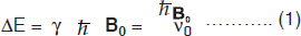
where, ν0 = (γ/2π)B0, is the frequency of electromagnetic field. Applying a magnetic field B1 perpendicular to the main static field cause rotation of the macroscopic magnetization. That is, with the application of a RF field, the nuclei are flipped from a parallel to an anti-parallel state. After the pulse, the nuclei return to the parallel state emitting RF energy, which is detected. This relationship is readily expressed by a simple Larmor equation
where ω0 (=2πν0) is the Larmor precessional frequency of nuclei in megahertz (MHz), γ the gyromagnetic ratio which is different for different nuclei and B0 the external magnetic field in Tesla (1 Tesla = 104 Gauss).
MR frequencies occur in the radio-frequency (MHz) range and the exact value depends on the strength of the externally applied magnetic field and the nucleus under investigation. The gyromagnetic ratio is a constant for a particular nucleus allowing observation of magnetic resonance to be easily tuned to a particular nucleus. Although MRI deals primarily with the population of hydrogen nuclei, other nuclei present in biological systems can also exhibit the magnetic resonance phenomenon. They are characterized by having an odd number of nucleons (protons or neutrons) and have associated gyromagnetic ratios as given in Table 1.1.4
Free Induction Decay (FID) and Fourier Transform (FT)
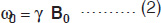
The magnetization arising from different number of nuclei (say proton) present in tissues is the so-called net (or bulk) magnetization M0 (=Mz) which is parallel to the external magnetic field, B0. A strong radio-frequency field B1 applied along x-axis, tips M0 away form z-axis (Fig. 1.2A). The duration and power of the RF pulse determines the direction of M0 after the pulse. If a so-called 90°x or π /2 pulse is applied, M0 points along the positive y-axis (Fig. 1.2B), i.e. the z-magnetization (longitudinal) is now transferred into a transverse plane. The Larmor frequencies of the various (proton) nuclear magnetic moments vary and as a consequence, the vector M (actually Mxy) now splits into its components (Fig. 1.2C) in the xy plane and produce a voltage signal. A plot of the time dependence of the intensity of the y-component of the Mxy magnetization (that is, the voltage induced in the receiver coil) as a function of time is known as free induction decay, FID (Fig. 1.2G). Thus, FID represents the time evolution of the transverse magnetization. It is necessary to analyze this time-domain signal f(t), into its individual frequency components, F(ω). This is accomplished by a mathematical formulation, known as the Fourier transformation (FT), which is given by

This allows not only the extraction of the individual frequencies but as well as their associated amplitudes, which are proportional to the spin density at a particular spatial location (Fig. 1.2H).
The frequency of the energy depends upon the strength of the magnetic field of the MRI scanner. By manipulating the magnetic field strength across the body, different tissues of the body can be labeled with different radio frequencies (vide infra). The sum of these frequencies is detected, sent back to the computer and analyzed to produce images. Most clinical MR images rely on the abundant and strong signal of mobile hydrogens in the body that arise primarily from water and fat. The images are pictorial representation of the spatial distribution of these mobile protons. The density of mobile protons in tissues affects the image contrast in addition to other factors discussed later in this article. For in-depth details of the physical principles of MR, the reader may refer to standard textbooks and review articles10–19.5
Fig. 1.2: Spin magnetization rotated away from the main magnetic field (Bo). (A) By the application of an RF field B1 along the x– direction, the magnetization (Mxy) is rotated to y–direction (B). Thereafter, the nuclei (spins) continue to rotate in the transverse plane at different rates, (C), (D), (E), causing their resultant magnetization Mxy to diminish (T2 process). Meanwhile spin-lattice relaxation (T1) process causes the nuclei to realign along Bo(F). (G) the free induction decay (FID) resulting from T2 process and its Fourier transform (H).
Relaxation and Contrast
With the RF switched off, the macroscopic magnetization will get back into the original position by a process called relaxation. Initially, the nuclei are in thermal equilibrium with the static field B0 (along z-direction magnetization, M0 = Mz) when they are completely aligned (Fig. 1.2A). After RF excitation, the nuclei are disturbed and have tendency to get back to the original thermal equilibrium by realigning (Fig. 1.2F) with B0. The time constant that describes the rate, at which the z-component of the net magnetization (Mz) returns to its equilibrium value M0, is the T1 relaxation time. This happens due to the excited nuclei losing its energy to the surrounding molecular environment, called the ‘lattice’, hence spin-lattice relaxation. The recovery of z-component of the magnetization (Mz) is given by6

where M0 is the initial magnetization and ‘t’ is the elapsed time from the start of the FID. In MRI, signals are repeatedly generated by the application of a series of 90° RF pulses, which establish a ‘steady state’ magnetization. With the constant repetition time (TR), the signal is given by

This effect is called ‘saturation’ and is the basis of T1 contrast.
Second phenomenon is the interaction between spins within a group causes the macroscopic magnetization to dephase, which is denoted as T2, the spin-spin (transverse) relaxation time. This refers to the loss of energy due to interaction with other nuclei aligned with the magnetic field. Immediately after the 90° RF pulse, the net magnetization is transverse to B0 field, i.e. along the xy plane (Fig. 1.2B). All the nuclei making up their transverse magnetization (Mxy) are momentarily phase-coherent, and form the signal FID. T2 represents the time constant associated with the loss of this signal (magnetization Mxy) in the xy plane (Fig. 1.2E). It is a decay process involving the loss of energy (or phase coherence) by the nuclei because the nuclei are interacting with each other. T2 relaxation is actually confounded by T2* relaxation, which is much shorter and results from inhomogeneities in the magnetic field. T2 relaxation time is normally measured with a spin echo (SE) pulse sequence involving multiple echoes (Fig. 1.2). The relation of the peak height of a spin echo at time TE to the peak height of a FID [Mxy (0)] is

Applying additional 180° RF pulses at time t = 3TE/2, 5TE/2, …. creates additional spin echo signals with peaks at times t= 2TE, 3TE …. The number of echoes observed is limited by the T2 decay.
Most MR images are either T1- or T2- weighted (vide infra). T1 and T2 refer to magnetic resonance time constants that are intrinsic to a given tissue. T1 and T2 have been separated for purposes of discussion, however, it is important to realize that they are occurring simultaneously during any given imaging procedure, and both are contributing some relative amount to the imaging process. T1 and T2 are specific tissue characteristics and their value will vary depending on factors such as magnetic field strength. Nevertheless, at a given field strength, different tissues have different characteristic T1s and T2s (Table 1.2).
|
The primary sources of inherent tissue contrast in MRI are three-fold: proton (spin) density (PD), T1 and T2. Unlike PD which may vary by just a few percent between various tissues, T1 and T2 relaxation times can vary as much as more than 100% among soft tissues (Table 1.2), and can have important effect on image contrast (Fig. 1.3). For example, the T1 of CSF is several times greater than white matter. Similarly, edema has higher T1 and T2 than normal white matter. Few types of lesions, such as lipomas, melanomas, and fibrous lesions deviate from this general rule of having higher T1 and T2 values than the surrounding normal tissues. Although data on proton density are limited, it often occurs that PD values are also directly correlated with relaxation times. For example, normal tissues or lesions having longer T1 and T2 values also tend to have higher PD values as has been demonstrated for brain white matter lesions20 and appear to be generally true for most other lesions.
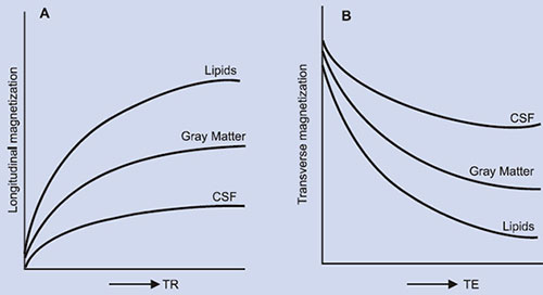
Fig. 1.3: Relative MR signal intensities of tissues: (A) as a function of the repetition time (TR) and (B) as a function of the echo time (TE).
The pixel intensity in a MR image is a function of T1, T2 and image acquisition parameters (vide infra) such as TR (time of repetition) and TE (time of echo). In routine MRI, the images obtained are either PD, T1-weighted or T2-weighted. They usually do not refer to images that display PD, T1 or T2. Instead, the terms refer to the relative weight with which the three parameters affect the tissue contrast in MR images. Such images are obtained by varying the parameters TE and TR. Generally, tissues with short T1 will appear bright on T1- weighted image, and tissues with long T1 will appear dark. For example, in a T1- weighted image of the brain, the fat will appear as white; white matter as light gray and gray matter as gray and the CSF as black as shown in Figure 1.4A. In T2-weighted image of coronal section of the brain (Fig. 1.4B), fat appears as gray while the white matter as dark gray; the gray matter appears as gray and the CSF as white. T1-weighted images are useful for viewing the anatomy (morphology) while T2 images are useful for identifying the tissue pathology.
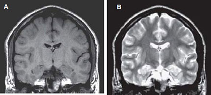
Figs 1.4A and B: Coronal SE MR images of a volunteer: (A) T1 – weighted [slice thickness = 5 mm; TR = 550 ms; TE = 15 ms; field of view (FOV) = 250 mm] and (B) T2- weighted (slice thickness = 5 mm; TR = 2600 ms; TE = 90 ms; FOV = 250 mm).
MR images are produced by assigning shades of gray, white, and black to the strength of the signal produced by the relaxing protons. Diffusion-weighted imaging (DWI) is a technique that generates tissue contrasts that are based on completely different phenomenon than those that are involved in conventional MRI technique. Diffusion techniques are based on the amount and direction of Brownian movement of free water protons; further details are presented later in this article.
Magnetization transfer (MT) is yet another method by which tissue contrast can be manipulated. MT is based on the principle that protons exist in essentially two pools, the free form and bound form, their magnetization can be transferred. By transferring magnetization from one pool to another, it is possible to design pulse sequences to produce substantial changes in tissue contrast. The common use of this phenomenon is in the brain to visualize better peripheral vasculature by improving the saturation of background tissue. In addition, recurrent meningiomas and basal ganglia calcifications has become more evident with the use of MT.
Static Magnetic Field and Gradients
The quality of MRI systems has been available since the early 1980s have improved exponentially in recent years. Although the early systems used resistive magnets, super conducting magnets are now standard. MRI scanners are generally characterized by the strength of the magnetic field. Most imaging procedures are performed with field strengths in the range of 0.2 to 1.5 Tesla, although imaging outside this range is possible. Larger field strengths permit shorter imaging time and improved resolution. The strength of the magnetic field determines the tissue (proton) resonant frequency. This is the frequency that is receptive to the RF pulses applied to the tissue and is also the frequency of the RF signals emitted during the imaging process.
Prior to actual imaging, the magnetic field is same at all points throughout the patient's body. However, during acquisition the gradient coils are switched on in a pulsed fashion. The fundamental principle of image formation is that the MR signal frequency, eq. (2), can be made to depend linearly on the spatial location of the group of nuclei producing the signal14 by applying moderate linear gradients. For the imaging experiment, eq. (2) is modified to

where ωi is the frequency of the proton at position ri and G is the vector representing the gradient amplitude and direction. It is, therefore, easy to see how a 1-D image projection is made. The signal is acquired in the presence of a field gradient and the intensity is plotted against the frequency6, with the frequency axis being ‘coded’ for, i.e. be proportionately equivalent to the spatial position. Images in two or three dimensions are made by an extension of this coding concept, using additional magnetic field gradients along the y- and z-axes, and recognizing that a precessing spin experiencing a gradient pulse of duration ∆t along either of these axes will accumulate an additional phase, e.g.,

Gradient coils are situated within the bore of the magnet. A current is passed through the coils, which are designed to produce a linear change in the main magnetic field in each of the three axes independently. The purpose of these gradient magnetic fields is two-fold: slice selection and pixel localization within the slice. The combination of a field gradient inhomogeneity and excitation by a specific frequency permits slice selection. The presence of a gradient field during relaxation helps to localize the protons within the slice that was selected during excitation.
The steeper the gradient field, the thinner will be the slice. Similarly, narrow bandwidth RF pulses, produces thinner slices. The gradient coils consist of three pairs: x-gradient, y-gradient and z-gradient. z-gradient (Gz or Gs) changes the gradient magnetic field along the z-axis thereby allowing a slice of the patient to be selected for imaging. x-gradient coils produce a magnetic field gradient across the patient and therefore the horizontal axis across the patient, thus providing spatial localization along the x-axis of the patient. This technique is usually called ‘frequency encoding’ (Gx or Gf). The y-gradient coils produce magnetic field gradient through the patient from front to back, and by convention, the y-axis is the vertical axis through the patient used for ‘phase encoding’ (Gy or Gp) the NMR signal. Together, the y- and x-gradients allow precise determination of where within the imaging plane the contribution to the NMR signal from each voxel or pixel originates. The z-gradient is always used for selection of a transaxial plane to be imaged and is called ‘slice selection’. To select either the axial, sagittal or coronal plane for imaging, the z-, x- or y-gradients, respectively, will be energized as magnetic fields add vectorially. When all the three gradients are energized at the same time, an oblique plane is defined. In an actual imaging procedure, once a plane is excited by a selective irradiation in z-axis, a gradient is applied along the x-axis during signal acquisition and thus a projection is obtained along the x-axis. From this point on, all projections are obtained along the x-axis but a y-gradient of increasing strength is applied to each projective sequence. This process encodes the y-axis spatial distribution and in fact an FT decodes the information.
RF Pulse Sequences
A pulse sequence is a series of timed events involving RF pulses, gradient pulses and digital sampling of an analog signal. It accomplishes two tasks: (i) to collect the data in an orderly fashion so that the origin of the signals can be determined – i.e., the pixel 10position – and this is the function of the gradient magnetic fields outlined earlier; and (ii) it influences the image contrast – pixel character – by specifying the timing and power of the RF pulses. Many of the parameters that have to be specified in a pulse sequence, such as the timing and magnitude of gradient magnetic fields are included in the computer software.
In general, MRI sequences are divided into simple building blocks that control slice selection, frequency encoding, and phase encoding of the 2D or 3D space. Hundreds of sequences exist and they all have some elements of these building blocks in common. These may be categorized into two main groups built around either the spin echo (SE) or the gradient echo (GE) and the images acquired in either a single echo or a multi-echo approach10, 19, 21. The SE pulse sequence shown in Figure 1.5 is often used in clinical diagnosis. The basic sequence of events in SE is a 90° RF pulse excitation, spatial encoding, a 180° refocusing pulse, and signal readout. The pulse sequence diagram contains several labeling conventions and in order to get images with good contrast and quality, one needs to specify (a) type of pulse sequence, (b) time intervals TR, TE, etc. (c) matrix size, (d) number of signal averages, (e) plane of image, (f) spatial separation of the slice, etc. The signal intensity, S may be given by10

where C is a constant related to the amplification of the MRI receiver, and Mz reflects the proton number density. For short echo times (TE), eqn. (9) simplifies to

Multislice and multiecho techniques help to decrease total scan time.
The other most commonly used sequences are partial saturation, inversion recovery (IR), STIR, FLAIR, etc. IR sequence provides heavily T1-weighted images, is often effective in defining small lesions or the internal structure of lesions where detectability may involve only subtle differences in T1 values and is designed to minimize T2 relaxation.
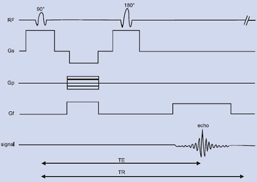
Fig. 1.5: Spin echo RF pulse sequence showing the various time delays such as time of echo (TE), time of repetition (TR), etc. Gf, Gp and Gs refers to the gradient field applied along x, y and z-axes. “Echo” refers to the NMR signal (FID).
Measurement times are long due to incorporation of long TR values plus the inversion time (TI) component in to the sequence. Tissue signal suppression may be observed using STIR (short tau inversion recovery), a special case of IR sequence. By using a short TI, images with suppression of signals from specific tissue types, such as fat, can be achieved. In STIR, the idea is to wait only until the fat signal crosses the null point (0.69 × T1), the time at which there is no fat signal available to be flipped to the transverse plane. A variation of STIR is FLAIR (fluid attenuated inversion recovery) and in this sequence, rather than using a short TI value, a very long TI is used to catch water at the null point. This results in suppression of structures such as ventricles (CSF) and has been shown to help to define even very small demyelinating lesions such as multiple sclerosis (MS). The drawback of FLAIR lies in the fact that TR value greater than 5000 ms are required with TI values of about 2000 ms, thus increasing the measurement time.
Fast Imaging Sequences
The SE pulse sequence has been the fundamental platform for MR imaging. However, sometimes measurement times are long and the sequence is sensitive to motion artifacts and thus becomes unsuitable for many sick patients. There are several reasons to acquire MRI data quickly and the principal impetus is to improve clinical efficiency. In addition, to minimize patient discomfort and the adverse effects of involuntary physiological patient motion on image quality. Finally, shortening of scan time can open many new avenues for dynamic scanning such as cardiac imaging, functional studies like task activation, etc. The methods for reducing the measuring time as proposed by various groups can be divided into two categories. First, using gradient echoes and the second one based on a different phase coding of signals (echoes) recorded within one pulse sequence (mostly CPMG sequences) after one single excitation of the spin system. GE sequences use a small flip angle for excitation, followed by a gradient reversal instead of the 180° RF pulse for echo formation, which is applied in the read out direction (Fig. 1.6). These methods require highly homogeneous B0 field. By employing gradient reversal it is possible to achieve shorter echo times of the order of TE = 1 or 2 ms. In addition, it is possible to use a short flip angle which helps to use shorter repetition times. FLASH (fat low angle shot)22 is one such sequence, which uses a flip angle of 15 to 30° instead of a 90° pulse. Another method that is also based on GE is FISP (fast imaging with steady state precession)23. In FISP the slice gradient, the phase encoding gradient and the read gradient are always switched on a second time with equal duration but opposite sign, so that finally all spins are again in the same position they were at the beginning. In this way, dynamical steady state is reached for the longitudinal as well as transverse magnetization. Also, GE sequences have increased contrast sensitivity over SE sequence due to increased T2* dependence.
Echo-planar imaging (EPI)24 is yet another approach to rapid scanning which is widely used for image data acquisition in very short time scale, typically less than 100 ms. EPI acquires a complete set of GEs with a single shot (Fig.1.7) or in a series of multiple shots.


Fig. 1.7: Single–shot echo-planar imaging sequence. Following a selective excitation, multiple gradient echoes are generated.
EPI is a ‘snap shot’ sequence to map the multiple phase-echoed lines of k-space with a single RF excitation, i.e. a complete data set is acquired to reconstruct an image from the MR signal produced by a single RF excitation of the selected slice. The original concept and its early realtime biomedical application employed a continuous scan path, zigzagging rectilinearly through the entire k-space plane. This 13requires a clever manipulation of the encoding gradients Gf and Gp. Gf is inverted after each line-scan while Gp is applied very briefly in ‘flips’ after completion of a line. The inversion of a gradient actually inverts the scan direction in k-space. The gradient Gf is strong and rapidly switched to obtain very fast echoes, while the gradient Gp is flipped as narrow pulses coinciding with the zero crossings of Gf. These gradients are programmed to act in synchrony, generating a fast zigzagging route through k-space. The MR signal is continually sampled during this k-space traverse, and the method is therefore very fast and efficient.
The EPI technique may be implemented in either the SE or the GE version. If an 180° pulse is applied between the initial excitation pulse and the start of sampling, the sequence becomes SE EPI. The S/N is relatively poor in EPI. Each line must be digitized within a very short time, since all lines have to be scanned before the T2-decay of the spins following the RF pulse excitation. Short acquisition time for each line requires a large receiver bandwidth (BW) and, consequently, noise is higher. Spatial resolution is also usually limited.
The hardware necessary to collect good EPIs requires both strong eddy current-free gradients with rise and fall times of few millisecond and fast analog-to-digital converters (ADC), which can sample repeated GEs (with typical durations of 400 µs to 1 ms) over the 32 to 128 ms sampling time. With improvement in gradient coil technology, EPI can acquire a series of images within seconds, making bolus tracking, quantitation of diffusion, flow parameters and functional task activation (fMRI) readily imaged in realtime. However, EPI techniques are far more demanding with regard to artifact suppression. Susceptibility artifacts, chemical shift artifacts, and increased spin dephasing of flowing blood because of longer effective TEs are but some problems which are normally encountered. EPI sequences are useful in functional MRI, bolus tracking, diffusion and perfusion studies25, 26.
Another strategy for reducing measuring time is based on SE like RARE sequence (rapid acquisition with relaxation enhancement)27. Here the emphasis is not to reduce the repetition time, but rather to record a series of values of phase coding gradients simultaneously with one excitation of the spin system by different phase codings of different echoes. RARE is similar to conventional SE but typically uses many more echoes than conventional schemes, with 4 to 16 echoes acquired. Moreover, all the echoes are differently phase coded so that for 256 phase codings, only 32 excitations instead of 256 are required; this is a time saving of a factor of 8. There are several fast and other advanced pulse sequences for variety of disease purposes and some of them are described in detail in Chapter 3 of this volume.
Parallel Imaging
Most of the fast imaging sequences in use like EPI, FLASH, etc achieve their speeds by optimizing the gradient strengths, the switching rates, and the patterns of applied gradients and pulses. Beyond a certain threshold, however, rapidly switched gradients are known to produce neuromuscular stimulation, while excessively dense RF pulse trains can lead to unacceptable levels of RF energy deposition and heating of the tissue. The common feature of all the fast imaging sequences is that they all acquire data in a 14sequential fashion. The MR signal is always acquired one point and one line at a time, with each separate line of data requiring a separate application of field gradients and/or RF pulses. Hence, the imaging speed is generally limited by the maximum switching rates compatible with scanner technology and patient safety.
A new paradigm recently has been demonstrated called ‘parallel imaging’ to increase imaging speeds beyond the basic limits described above. In ‘parallel MRI’, multiple MR signal data points are acquired simultaneously, rather than one after the other. Parallel imaging require the use of multiple distinct detectors, with each detector providing some component of distinct spatial information to the image. In MRI, the spatial encoding accomplished by gradients can be replaced instead to array of RF coils. Thus with the use of array of coils and in combination with appropriate reconstruction strategies to encode and detect multiple MR signals or image components simultaneously, it is possible to increase the speed of existing image sequences without increasing the gradient switching rate or RF power deposition.
In 1997, simultaneous acquisition of spatial harmonics (SMASH) method28 was introduced for accelerated MR imaging using parallel imaging strategy. The SMASH technique uses linear combinations of component coil signals from a surface coil array to replace time consuming phase encoding gradients28. Later another methodology called SENSE (sensitivity encoding technique) has been proposed29.
Image Processing
The MR signal produced through the use of RF pulse sequences (vide infra) cannot directly be translated into an image. It is necessary to convert from a frequency representation to a location representation. A digital computer, with sufficient memory and storage, performs necessary operations for this conversion (transformation). There are numerous ramifications of the imaging technique, such as (a) sequential point technique, in which a single volume element is selectively excited and observed at a time; (b) sequential line technique, where an entire line of volume elements is excited and observed simultaneously with increased sensitivity compared to the earlier methods; and (c) sequential plane technique, where the sensitivity is further increased when an entire plane of volume of elements is excited and observed at once. The last of these is most widely used in clinical imaging. The variants of this technique are: the projection reconstruction, Fourier imaging, spin-warp imaging, and rotating frame imaging.
Two-dimensional (2D) FT imaging samples a line at a time in only one direction of sampling of the frequency representations. The direction of sampling is determined by the direction of the phase-encoding gradient. The information along this line is determined by using the frequency encoding gradient. When the entire frequency representation of the image has been sampled by repeated cycles of the 2D FT process using different phase-encoding gradient strengths, the sampled frequency representation is converted to an image in the computer by using a two-dimensional Fourier transform. Thus the FT has to be performed twice: first, along the x-axis and then along the y-axis and hence the name 2D FT technique.15
In addition, multi-section 3D imaging is also possible. In 3D imaging, the 2D FT process is repeated ‘n’ times without section selection, each time with a different value after z-gradient applied prior to read out of the FT direction. This process encodes z-axis information in exactly the same way it encoded along the y-axis. Further details about FT imaging are presented in Chapter 2 of this volume.
Magnetic Resonance Angiography (MRA)
In the past few years, magnetic resonance imaging of flow has blossomed into a powerful technique to visualize blood flow in vessels (Fig. 1.8). This technique called as magnetic resonance angiography (MRA), proved to be a valuable tool for evaluating vascular diseases30. In addition to its ability to image vascular anatomy, new, non-invasive approaches for measuring blood flow have in fact expanded the role of MRI in diagnosing vascular pathology such as, cardiac abnormalities, renal blood flow, etc. In MRA, blood vessels are rendered, not in the usual topographic format of standard MR images, but as a projection over a large volume, similar to a conventional angiogram. No external contrast agent is required because moving protons serve as intrinsic flow markers. MRA enables visualization of normal, laminar blood flow within the vascular system and its disruption due to any pathology such as a thrombus (blood clot). Also, MRI can be of particular use in evaluating vessel patency. Present practice is to use the so-called ‘bright-blood’ technique; i.e. signal from flowing protons is enhanced relative to the stationary protons through the pulse sequence and measurement parameters. The bright blood depicts arteriovenous malformations, aneurysms, stenoses and other diseases. Bright blood MRA methodology can be divided into time-of-flight (TOF) and phase contrast (PC) techniques.
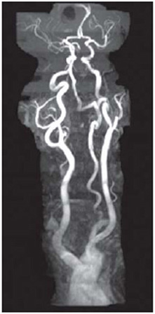
Fig. 1.8: MR angiography (MRA) of a patient showing the carotid arteries from aortic arch to circle of Willis.
MRA essentially envisages both arterial and venous flow through a certain volume of interest. To avoid an ambiguous diagnosis between these two types of flow, spatial presaturation pulses are applied to saturate the unwanted blood signal prior to its entry into the imaging volume. At the other limit, presaturation pulses can also be used in ‘black blood’ techniques where both arterial and venous blood signals are saturated out, and the vessels appear dark relative to the surrounding tissue. A common problem with MRA procedures is an exaggerated sensitivity to blood vessel stenosis. The stenotic region disrupts the laminar flow both in the area of, and distal to, the stenosis, causing signal loss from the imaged vessel. This can lead to an extremely variable appearance of the vascular lumina through which blood circulates. As the laminar flow is restored in the vessel, bright signal is seen again.
The different methods employed to produce MRA images are: 2D and 3D FT time of flight (TOF), 2D and 3D phase 16contrast (PC) and 2D FT cine angiography. 2D TOF method relies on flow-related enhancement to differentiate moving spins from stationary spins. A modified GE pulse sequence is used, as it is sensitive to flow. Blood flowing into the slice is fully magnetized (unsaturated) and gives higher signal than the surrounding (saturated) tissues. If the blood flow is perpendicular to the slice then maximum flow-related enhancement is achieved. If a blood vessel runs parallel along the slice the blood flowing within the vessel, being exposed to multiple RF pulses, soon becomes saturated, giving little or no signal. In a similar manner slow-flowing venous blood may become saturated within the imaging slice and so appear with lower signal intensity, compared with faster-flowing arterial blood. 2D TOF technique can be used for wide range of studies. These include evaluation of the carotid bifurcation, evaluation of the pelvic view for deep vein thrombosis, evaluation of lower extremities, investigation of suspected basilar artery occlusion and suspected intracranial venous thrombosis, and cortical venous mapping30. 3D TOF acquires a whole three-dimensional volume or slab of tissue with saturation of the stationary tissue and flow related enhancement from blood entering the slab. Advantage of 3D TOF is the use of very thin slices, an increase in the SNR, and reduced sensitivity to turbulence and pulsation. The clinical applications include the visualization of arteriovenous malformations, aneurysms, venous angiomas, carotid occlusion, thoracic vessels and abdominal vessels.
Two-dimensional phase contrast angiography (PCA) uses velocity-induced phase shifts to distinguish between flowing blood and surrounding tissue. A slice of tissue is excited by the application of a RF pulse followed by two equal but opposite “bipolar” gradients. Protons moving along the direction of the bipolar gradient experience phase shifts between the application of the two gradients, while the stationary tissue does not. PC angiography is based on these phase shifts. The size of the phase shifts depends upon how far the flowing protons have travelled between the application of the bipolar gradient pulses. Faster-flowing protons will demonstrate greater phase shifts. When the amplitude of the bipolar gradient pair is inverted, a second acquisition is made and this causes a phase shift in the flowing protons opposite to the first.
The clinical applications of 2D phase contrast angiography include investigation of occlusion of the basilar artery, dural sinuses, intracranial venous structures, portal venous system, etc. In 3D PC the data are acquired with additional phase encoding in the slice select plane/direction, in a similar manner to 3D TOF. Clinical applications include evaluation of aneurysms and arteriovenous malformations, demonstration of venous thrombosis, etc.
Recently contrast enhanced (CE) MRA has emerged as a new tool, which is advantageous in situations of tortuous vessels and stenotic regions. Due to the fact that gadolinium and other transition and lanthanide based contrast agents has no nephrotoxic potential its use in kidney studies is widely accepted. Depiction of large aneurysms is markedly simplified with CE-MRA compared to DSA. The main advantage of CE-MRA compared to TOF and PC MRA is its intrinsic advantage in acquisition speed. The detailed role of magnetopharmaceuticals for enhancement of MRI contrast is discussed in Chapter 10 of this volume.17
Diffusion and Perfusion Imaging
Diffusion-weighted MR imaging (DWI) is used to map as well as assess and/or quantitate the microscopic motion of water protons in tissues31, 32. Measuring molecular diffusion may bring several potential useful new approaches to tissues characterization and functional studies. Microscopic motion of water protons namely randomly directed Brownian motion or diffusion might be used as a potential contrast mechanism. For motion in one direction, the mean translational distance, <L>, that a water molecule would diffuse in time ‘t’ is given by the so-called Einstein equation

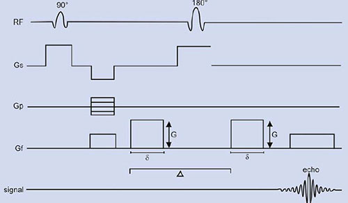
where D is the diffusion coefficient of water. The effect of diffusion on the MR images may be understood using a SE sequence in which a pair of bipolar field gradient pulses is included (Fig. 1.9). The purpose of these gradient pulses is to magnetically ‘phase tag’ the diffusing spins, in much the same way a radiotracer is used to tag a molecule in the more classical diffusion studies in physiology31. In Figure 1.9, the gradient pulse amplitude and duration are denoted by G and δ, respectively, and the interval between gradient pulses by ∆.
For two spins (a1 and a2) diffusing past each other, the first gradient pulse induces a phase shift of the spin transverse magnetization depending on the spin position a1 (spin tagging). Likewise, the second gradient pulse will produce a phase shift, which depends on the spin position a2 at this time (spin untagging). Due to the 180° RF pulse, the net phase shift will be

For static spins (a1 = a2), the bipolar gradient pair has no effect on phase. For moving spins, however, there is a net phase change, which depends on the spin history during the interval ∆ between the gradients that affects the transverse magnetization.
Consider now the macroscopic magnetization arising from the vector sum of the individual diffusing spins, which have different displacement histories (i.e. different phase shifts). Interference between their phases results in attenuation S/So (<1) of the signal amplitude which, for the diffusion process, is given by:


where b is the ‘gradient factor’ characterizing the strength and duration of the applied diffusion gradients and is defined as
Diffusion coefficients, or diffusion lengths, may be evaluated by varying either G or δ and by measuring the slope of the semi-logarithmic plot of (S/So) vs (Gδ)2.
In tissues, water interactions and collisions with macromolecules and membranes usually limit diffusion; hence in biological studies the diffusion coefficient values are quoted as apparent diffusion coefficients (ADCs) which is defined as:

The local environment influence diffusion; e.g. in areas of white matter there is greater diffusion along the myelin sheaths than across them. Therefore, the diffusion of water in tissues is anisotropy; i.e. there are different apparent diffusion coefficients in each direction. In fact, diffusion is a three-dimensional process and the molecular mobility may not be the same in all directions. This anisotropy may result from the physical arrangement of the medium or from asymmetric disposition of obstacles that limit diffusion. In fact, diffusion is a tensor, an array of numbers that describe mobility rates in different directions. Diagonal elements Dxx, Dyy, and Dzz represent molecular mobility in the three directions x, y, and z-axis. The non-diagonal elements, such as Dxy, Dxz, or Dyz, show diffusion in one direction is correlated with some molecular displacements in a perpendicular direction. Molecules can diffuse in all three dimensions and hence diffusion tensor mapping becomes more useful. Diffusion is a major advance in the continuing evolution of MR imaging. It provides contrast and characterization between tissues at cellular level that may imply differences in function31–33. DWI is useful in the early detection and characterization of cerebral ischemia and renders this technique ideal for evaluation of stroke management31, 34–36.
Perfusion-weighted MRI (PWI) measures blood flow, which is different in many brain and cardiac disorders31, 37. PWI is useful to demonstrate the microscopic vascular proliferation (neovascularization) associated with tumor growth. Tissue perfusion is normally assessed following a dynamic injection of contrast material, gadolinium diethylene triamine pentaacetic acid (Gd DTPA). For example in cerebral tissues, Gd is restricted to the intravascular space. Gd being paramagnetic creates microscopic field gradients around the cerebral microvasculature, resulting in a change of T2 19relaxation and signal loss (vide infra). From the amount of signal loss, the concentration of gadolinium in each pixel can be calculated, and a pixel by pixel relative estimate of blood volume can be inferred. Maps of cerebral blood volume (CBV) and CBF can be generated. As a rule, high-grade tumors have higher CBV values than low-grade tumors; and CBV values correlate with the grade of vascularity and mitotic activity. Knowledge of tumor vascularity is helpful to improve tumor grading, to identify optimal biopsy site in tumors with heterogeneous vascularity, to monitor for malignant degeneration and treatment efficacy, and to differentiate tumor recurrence from radiation necrosis. Similarly, PWI of myocardium is a useful modality to detect perfusion defects at rest and under stress. Contrast enhanced (Gd DTPA) PWI can be reliably used for assessment of myocardial perfusion in patients with ischemic infarcted myocardium. The uptake of contrast will be attenuated, in amplitude and rate, in regions of compromised flow.
Functional MRI
MRI can also be used to map changes in brain hemodynamics that correspond to brain functions. The ability to observe precise anatomical structures and also which structures participate in specific functions is due to a technique called ‘functional MRI’ (fMRI). fMRI provides high resolution, noninvasive report of the neural activity detected by a blood oxygen level dependent (BOLD) signal38–40. It is based on the increase in blood flow to the local vasculature that accompanies neural activity in the brain. These results in a corresponding local reduction in deoxyhemoglobin because the increase in blood flow occurs without an increase of similar magnitude in oxygen extraction41. Since deoxyhemoglobin is paramagnetic, it alters the T2*-weighted MR image signal. Thus, deoxyhemoglobin is some times referred to as an endogenous contrast-enhancing agent, and serves as the source of the signal for fMRI. Using an appropriate imaging pulse sequence, human brain functions can be observed without the use of exogenous contrast enhancing agent in many clinical MR scanner (field 1.5 T or greater). Functional activity of the brain determined from the MR signal has confirmed known anatomically distinct processing areas in the visual cortex42, the motor cortex43, 44, and Broca area of speech and language related activities45. The ability to directly observe different brain functions opens an array of new opportunities to advance our understanding of brain organization, as well as a potential new standard for assessing neurological studies and neurological risk46, 47 and the recent advances and applications of fMRI are presented in greater detail in Chapter 9 of this volume.
Contrast Enhancement with Exogenous Agents
In general, the MR properties of the tissues and their microenvironment are themselves capable of providing tissue contrast, however, manipulation of the signal intensities by external exogenous contrast agents is necessary in a variety of clinical situations to improve contrast between tissues with similar relaxation times in the normal and diseased states. The mechanism of contrast enhancement is related to several parameters: the class of contrast media (paramagnetic or superparamagnetic), their concentration within the tissue, their compartmentalization in various physiological 20and pathophysiological spaces, and the weighting of the imaging pulse sequence used. Thus, formulations that shortens either the tissue T1 or T2 relaxation time has been devised. The T1 shortening agents are hydrophilic chelated paramagnetic metal ions such as Gd3+ and Mn2+ that have unpaired electrons and behave as molecular magnetic dipole moments. The fluctuating magnetic fields caused by the tumbling molecular dipole moments alter the T1 of tissue water protons. The paramagnetic ions may be chelated to a wide variety of molecules to reduce toxicity and to retard the free tumbling rates of the metal ion centers thereby enhancing their relaxation effects on the tissue protons being imaged.
Another class of contrast agents are the ones that alters the tissue T2 (or T2*) values by inducing local magnetic field gradients in cells. As the tissue water protons diffuse through these induced field gradients, their MR signal is attenuated. Superparamagnetic materials such as magnetite particulates are representative of this class which are taken up by phagocytosis and clustered within lysosomes intracellularly. Several superparamagnetic iron oxide formulations (SPIO, USPIO) have been used as T2 contrast agents for enhancing liver, spleen and bone marrow lesions because they are selectively absorbed by the reticuloendothelial systems of the tissues. MR contrast agents may be broadly grouped, in terms of their bio-distribution, as being intravascular, extracellular, or organ specific which are based on the type of chelation, packaging (i.e. liposomal, viral, encapsulated) or coating (e.g. antigen-specific) surrounding the paramagnetic ions or particles.
Gd3+ chelates administered intravenously either as a continuous infusion or as a bolus injection, are available both in ionic and nonionic formulations. The most common ionic agent uses Gd3+ ion and diethylaminetriaminopetaacetic acid (DTPA) as the chelating agent. This is widely used in brain pathologies that alter the blood-brain barrier (BBB), and clinical utility is high in both neoplastic and non-neoplastic diseases. In pathologies affecting the BBB, e.g. an infarct, leakage of the paramagnetic agent across the disrupted tight junctions of the capillary endothelial cells delineates areas of increased cerebrovascular permeability. Disruption of the BBB caused by tumor, inflammation or edema is observed as an area of hyperintense signal on T1-weighted images. The nonionic formulation of Gd3+ chelate virtually accomplishes the same contrast enhancement as described above. The nonionic paramagnetic complex has no net charge to be counterbalanced at the expense of an increase of viscosity and osmolality, and this feature leads to the potential clinical benefit of higher dose injections. The role of magnetopharmaceuticals for enhancement of the MRI contrast has been presented in detail in Chapter 10 of this volume.
MRI of Other Nuclei
Imaging of nuclei other than proton is also possible such as 23Na and 19F. Such measurements are exacerbated by the low intrinsic sensitivity of these nuclei relative to proton and the low physiological concentrations relative to water. Sodium MRI studies has demonstrated that the method can be useful for monitoring edema development, cerebral redistribution of sodium following ischemia48 and myocardial infarction49. The technique has been found to be useful to detect early cartilage 21degeneration as well50. Since there is no MR visible fluorine in human body, the 19F MRI methodology depends on the exogenous addition of a fluorinated material. Perfluorocarbons that label vascular compartments at high concentration have been commonly used, especially in the assessment of vascularity and the kinetics of tissue perfusion51.
Recently, studies have shown that inhalation of hyperpolarized (HP) gas allows images of the human lung air spaces by MRI with excellent contrast resolution.52–58 Since conventional proton MRI yields very poor images of the lungs because they are filled with air and contain little water. Gases like 3He or 129Xe, both chemically inert noble gases with spin 1/2; are polarized by optical pumping before inhalation. Nuclear polarization up to 80% is achieved which corresponds to a huge polarization enhancement or hyperpolarization above the thermal polarizations obtained in standard MRI. Using helium imaging, normal and pathologic airway function can be seen in exquisite detail. Dynamic imaging of the inhalation and exhalation of hyperpolarized helium can sequentially delineate each segment of the airways. Helium is not absorbed by other body tissues so that just the airways are visualized. Promising clinical applications include evaluation of emphysema and asthma patients. In general, the method has immense potential applications in the domain of lung pathology and other perspectives in functional MRI.
IN VIVO MR SPECTROSCOPY (MRS)
Nuclei that have high natural abundance and sensitivity in living systems are most suitable for in vivo MRS. For these reasons, most of the applications of in vivo MRS have been using 1H and 31P nuclei10–12, 14–16. In living systems, there are two main sources of protons namely water and fat that are used for image formation in MRI. However, the protons of water and fat mask the signals of metabolites that are present in low concentration in tissues. Therefore, the detection of resonances of biochemicals with low concentration require special techniques for suppression of water signal, (vide infra). The aim of in vivo MRS is to obtain a spectrum that arises exclusively from the volume of interest (VOI), with the best achievable sensitivity and with minimum contribution from other regions. A multitude of localization schemes has been proposed; however, the techniques that are in clinical use today are limited. In this section the basics of various localization techniques are presented, for in-depth details the readers may refer to many excellent books11, 14, 16 available. The approach taken is to provide a brief overview of the observable metabolites in various organs using the various acquisition methodologies with special reference to proton MRS.
In vivo MRS began with the study of isolated tissues and surface regions from intact animals before the availability of gradients for MRI, which led to the development of localization techniques that obtain spectra from single volume of tissues. The basic requirement of in vivo localized MRS, as pointed out earlier, is to acquire the signal from a particular VOI with optimal sensitivity. Table 1.3 presents a brief summary of some of the available localization techniques that are in clinical use today. Magnetic field gradients in either the B0 field as in imaging or in the B1 (RF) field are used for localization of a particular volume. One of the earliest methods for localization of VOI is to employ surface coils. In general, MRS requires a homogeneous B0 field for signal acquisition.
|
The early localization methods like rotating frame spectroscopy uses B1 field of the surface coil for localization. Methods like depth resolved spectroscopy (DRESS) use B0 magnetic field gradients and a frequency selective pulse for localization and the methods that are mostly employed in clinical settings include stimulated acquisition mode (STEAM), point resolved spectroscopy (PRESS) and image guided in vivo spectroscopy (ISIS). These sequences acquire spectra from a single volume (SV). Currently, multivoxel spectroscopic [chemical shift imaging CSI or spectroscopic imaging (SI)] methods are also available which are used to acquire spectra from many voxels simultaneously. Since, most of these methods use MR images to guide the VOI localization and are more often termed as image guided localization methods. The following sections provide a brief survey of some of the early localization methods and those that are commonly used in clinical setting.
Surface Coil MRS
Surface coil is a small circular loop of wire that is positioned adjacent (proximal) to a sample for excitation and/or detection and is positioned in such an orientation that a major component of B1 field generated by the coil is orthogonal to the B0 field.
Fig. 1.10: The pulse sequence for DRESS. The RF excitation pulse is applied in the presence of a magnetic field gradient.
Surface coil provides rough localization, i.e. metabolites in the sample close to the coil are detected with good sensitivity, whereas metabolites far from the coil are not detected4. In addition by varying the RF pulse length, spatial selectivity can be achieved. The disadvantages include extremely inhomogeneous transverse magnetic field, difficulty in assessing VOI that is below the surface and contamination of signals from extraneous tissues. For these reasons, surface coils are used with other techniques like the use of adiabatic pulses for precise localization and phased array surface coil with correction algorithm for inherent inhomogeneities in the signal reception profile.
Depth Resolved Spectroscopy (DRESS)
DRESS sequence shown in Figure 1.10 was developed by Bottomley et al59 is the first spatial localization technique employing magnetic field gradients and was successfully used to acquire localized 31P and 1H spectra from humans and animals. In this method, a single slice is excited by applying a slice selection gradient to the plane of the surface coil with a frequency selective RF excitation pulse to provide depth resolution. The observed volume is the intersection of the excited slice and the sensitive volume of the coil, and is approximately a thick disc. Spatial localization depends critically on the excitation pulse and the surface coil used for detection. In DRESS, the sensitivity reduces as a function of the distance from the cylindrical axis of the surface coil51. For observation of a deep organ, signals from the surface regions can be suppressed effectively but sensitivity of DRESS sequence is directly related to the depth of the selective pulse that poses a great limitation. Another problem with DRESS is that significant loss of signal occurs for metabolites with short T2 due to short delay of a few milliseconds 24between excitation and detection necessitated by the application of a gradient-refocusing lobe for acquisition.
Image Guided Single Voxel (SV) Methods
Localization methods are mostly image guided in that they use proton images to guide the placement of VOI. Hence, MR images are acquired in all the three planes and frequency selective RF pulses are applied during the application of a gradient. Prior to carrying out localized MRS, magnetic field gradient spatially encodes the resonance frequencies and the frequency selective pulse excites the spin distribution within the sample. Localization techniques may be categorized as single volume (or voxel) or multivolume. The position and size of the VOI are determined by the region bounded by the intersection of the three orthogonal planes and the actual shape would normally depend on the slice profiles of the selective pulses. There are different pulse sequences available in the literature and brief details of some of the most commonly used sequences for proton MRS like PRESS and STEAM are described here.
Point Resolved Spectroscopy (PRESS)
PRESS or double spin echo was proposed by two groups59, 60 is an adoption of the 1D DRESS technique to localization in 3D. For proton MRS, initially chemically shifted selective saturation (CHESS) pulses are needed to suppress the water resonance. Spatial localization is achieved by three frequency selective pulses applied in the presence of an orthogonal gradient (Fig. 1.11B). The localized VOI is at the intersection of the three orthogonal slices (Fig. 1.11A). The first 90° pulse is applied in the presence of gradient (e.g. along the x-axis) that selects a slice orthogonal to this axis.

Fig. 1.11: (A) A voxel that is defined by the intersection of three orthogonal planes (B) Timing diagram of a PRESS sequence. The initial CHESS pulses are to suppress the water signal. Slice-selective RF pulses excite three interacting orthogonal planes.
| |||||||||||||||||||||||||||||||||||||||||||||||||||||||||||||
The magnetization of the selected slice is allowed to precess during TE1/4 and is refocused by a second pulse applied in the presence of a gradient along an orthogonal direction (e.g. the y-axis). At TE1/4 it refocuses the magnetization in a slice orthogonal to this axis. Finally, after a free precession delay TE2/4, a second refocusing pulse is applied in the presence of a gradient along the direction orthogonal to the first two directions (z-axis). This last pulse refocuses the transverse magnetization from a slice orthogonal to the first two slices. Therefore the acquired signal results from the volume element common to the three slices, producing a three-dimensional localization in one single scan. PRESS offers the important advantage of a factor of two gain in S/N, although signals are T2-weighted and J-modulated. The VOI definition and localization in PRESS are inferior to other sequences such as STEAM since the slice profiles of the 180° pulses are often worse than those of a 90° pulse. Further, the power requirement for 180° pulses is twice that of a 90° pulse, which may cause RF heating of tissues. Another disadvantage is the lengthened minimum echo time that is an important limitation for metabolites with short T2.
Stimulated Echo Acquisition Mode (STEAM)
This method shown in Figure 1.12 uses three frequency selective RF pulses that are applied in succession in the presence of mutually orthogonal x, y and z-field gradients61, 62. Each pulse is of 90°, and the second 90° pulse brings the magnetization to the longitudinal direction where it remains for a time period TM. The echo time TE is independent of TM.
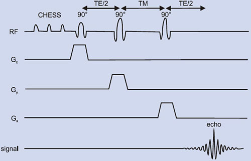
Fig. 1.12: Timing diagram of a STEAM sequence. The initial CHESS pulses are for water suppression. Here all the slice selective RF pulses are 90° and are applied with slice selection gradient each along one of the orthogonal directions x, y or z. Gradients in the sequence optimize the stimulated echo and suppress all other signals.
In all four echo signals are formed following the last RF pulse: one at TM arises from the second and third pulses, one at (TE/2 – TM) is formed by the first and second pulses, one at (TE/2 + TM) results from the first and third pulses and the stimulated echo is formed at the end of second TE/2. Gradients in the sequence are carefully set such that only the stimulated echo is acquired. All the unwanted echoes and the FID are suppressed using spoiler gradients. To achieve optimal efficiency each pulse should be 90°; however, it is not crucial to localization so long each of them is less than or equal to 90°. This reduces total investigation time and also since pulse angle can be less than 90°, the RF power deposition on tissues is less. However, whatever the nominal pulse angles, STEAM requires a complete dispersion of phases during the first echo delay and destruction of transverse magnetization during TM. The high quality localization obtained with STEAM has made it one of the most frequently utilized single voxel MRS technique despite the disadvantage that there is loss of a factor of two in S/N as compared to Carr-Purcell echoes. The water resonance is suppressed using CHESS pulses at the beginning of the sequence.
PRESS and STEAM differ in the nature of the echo signal. In PRESS, the echo is formed by refocusing the complete magnetization, whereas in STEAM, only part of the available signal produces the stimulated echo. Consequently, the signal-to-noise ratio is two times higher in PRESS compared to STEAM. STEAM is not well suited for observation of nuclei with short T2 values like 31P. In general, the T2 values for protons are much longer than the T2 values of 31P, and the use of STEAM has been primarily for localized proton MRS. Also, modulation from J coupling is reduced with short TE STEAM compared to short TE PRESS.
Multivoxel Spectroscopy: Spectroscopic Imaging (SI)
Single voxel spectroscopic technique can be extended to multivolume called chemical shift imaging (CSI) or SI63, 64. The spatial information (encoding) is accomplished by switched gradients of the B0 field.

The data in SI is collected in the absence of a readout gradient (Fig.1.13) to preserve the chemical shift information while in MRI readout gradient is used to obtain spatial information in one of the dimensions. Similar to the phase-encoding in MRI, a sequence of gradient values generates a complete set of spectra which can be spatially and spectroscopically resolved after multidimensional FT. Spectroscopic imaging procedures can be applied for 1D, 2D or even 3D acquisition of an organ. Since, localized spectra from many locations can be acquired simultaneously; SI is a more attractive method than single voxel techniques. The advantages of SI include acquisition of spectral data from small VOIs and the ability to reconstruct low-resolution metabolite images from the spectral data in which the pixel intensity is proportional to the relative concentrations of the metabolites. These metabolic maps or images are useful in visually assessing the spatial variation in the metabolite concentrations. EPI-based SI sequences are now available, which decrease image acquisition times.
However, the disadvantage of SI is that the signal from a voxel is prone to contamination coming from outside the VOI. This contamination occurs due to discrete and finite sampling, since the number of phase-encoding steps is typically more limited than normal imaging acquisitions. In addition, shimming the magnetic field over large volume of tissue and long acquisition times are other disadvantages. Gradient induced eddy currents and inhomogeneity in static magnetic field makes water suppression using CHESS pulse problematic in SI and leads to individual spectra being offset in frequency.
Recently in an effort to combine the advantages of both the SV and SI localization methods, while decreasing the disadvantage of either method, an approach to acquire in vivo data combining both SV and SI sequences are developed. The hybrid SV-SI pulse sequence is shown in Figure 1.14. Here, SV method is used to localize a relatively large VOI and phase-encoding gradients are used to subdivide the large VOI into smaller voxels. The advantage of SI localization from multiple voxels is retained, while the use of the SV method to preselect the large VOI greatly minimizes spectral bleed contamination from the outside lipid signals. The method allowed improved shimming, improved spectral resolution and water suppression. Several multidimensional experiments have demonstrated the potential of SI in the study of human brain65–68.
Water Suppression in Proton MRS
In MRI, images are obtained from the strong signals from the inherent high MR sensitive protons which are in high concentration in biological tissue. However, in proton MRS, detection of resonances from metabolites with lower concentrations in the presence of a large water proton signal is a major problem. The concentration of water in tissues is of the order of 70M compared to the millimolar (mM) concentration of other metabolites. Hence, there is the need for water suppression from the VOI and several methods have been developed that exploit the chemical shift differences between the water and the other metabolites69–71. The common one is to use chemical shift selective (CHESS) RF pulses72 which excite a limited narrow band (∼ 60 Hz) of RF frequencies corresponding to the water signal in the sample.
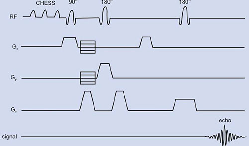
Fig. 1.14: Sequence diagram for hybrid spectroscopic imaging (SI) and single voxel (SV) technique that combines SV localization of a large VOI and two-dimensional SI.
In this method, one or more 90° RF excitation pulses are applied at the water signal and in addition ‘crusher’ gradients are used to eliminate the excited water signal in the transverse plane (Fig. 1.14). The other metabolites are given the RF excitation in the selected region and detected in the period when water magnetization is beginning to recover and not available for excitation. The efficacy of water suppression when using CHESS depends on B0 and B1 homogeneities and on T1 of water. B0 inhomogeneities can be reduced by optimized shimming and similarly B1 inhomogeneities may be eliminated by using adiabatic RF pulses. Most commonly used techniques of in vivo proton MRS like STEAM and PRESS, use CHESS pulses in the beginning of the sequence for water suppression (Figs. 1.11 and 1.12).
In in vivo MRS, often the spin echo signal is collected. STEAM and PRESS require the use of long echo times of 135 to 270 ms for adequate water suppression and to avoid instrumental problems, such as eddy currents due to the application of the magnetic field gradients for localization. Such long delays between the excitation and acquisition often results in dephasing the signals of the metabolites due to T2 relaxation. For metabolites with short T2 this can lead to almost complete loss of the signal. Therefore, the choice of TE in localization sequences is important for observing the metabolites of interest. The methylene protons of glutamate (Glu) and glutamine (Gln) are observed as complex multiplets at short TE's due to J-modulation. To observe the methyl resonances of lactate (Lac) and alanine (Ala) often longer TE's such as 135 and 270 ms are used to allow the signals to rephase. To observe metabolites like GABA and lactate, spectral editing techniques are sometimes used (vide infra). For TE's greater than two or three T2 intervals (e.g. mobile lipids), the use of shorter 30TE's can reduce the signal loss. In 31P MRS, since T2 of most of the phosphorus containing compounds is short, measurement of free induction signal is preferred to avoid the loss of metabolite signal.
APPLICATIONS OF IN VIVO MRS
Over the past decade in vivo MRS has increasingly been applied in clinical setup using nuclei like 1H and 31P to study the metabolism of several disease processes11, 15, 16 (see Chapters 11, 13–16). MRS can be carried out using different nuclei that include 1H, 31P, carbon (13C), lithium (7Li) and fluorine (19F). Using MRS it is possible to detect certain biochemicals that participate in different metabolic pathways. It provides information about energy status [phosphocreatine (PCr), inorganic phosphate (Pi) and nucleotide phosphates (NTP)], phospholipid metabolites [phosphomonoesters (PME), phosphodiesters (PDE)], intracellular pH and free cellular magnesium concentration through 31P MRS. Natural abundance or enriched 13C MRS provides information about glycolysis, gluconeogenesis, amino acids and lipids. Water-suppressed 1H MRS shows total choline (TCho), total creatine (TCr), lipids (Lip), glutamate (Glu), glutamine (Gln), inositols (Ins), lactate (Lac) and in brain, N-acetyl aspartate (NAA). 7Li and 19F MRS can be used to study pharmacokinetics and their applications are outlined in Chapter 18.
SUMMARY
Biomedical MR has achieved amazing level of success as an important tool through MRI and in vivo MRS to study several disease processes. MRI is a multiplanar imaging capability, has high spatial resolution, excellent soft tissue contrast, and uses no ionizing radiation. It covers a broad range of applications from fast noninvasive anatomical measurements, to studies on tissue physiology and metabolism. Since it is noninvasive, studying chronic diseases has several advantages for monitoring disease progression and therapy response. MRI is also useful for pharmacodynamic studies in humans to assess whether new compounds are exerting the desired pharmacological effects. Such studies will serve and guide the dose selection for the extensive and expensive clinical efficacy trials. MRI has also been developed as a powerful tool to guide interventional procedures in clinical medicine. Designs of new open magnet systems allow improved patient access for MR-guided interventional procedures with the use of MR-compatible needles and catheters. Applications of this interventional MRI include aspiration cytology, chemoablation, cryoblation, etc. As MR technology matures, the technological limits on the achievable scanning speed and pixel resolution are rapidly approaching the limits imposed by the laws of physics.
In vivo MRS can now be used as a unique means to probe the biochemistry of living systems with diagnostic importance. The goal of obtaining noninvasive biopsy information has pushed the development of several optimized localized MRS procedures with water suppression and editing techniques. The potentially powerful feature of in vivo MRS is the ability to measure endogenous metabolites noninvasively as well as changes in tissue metabolism. Besides 1H and 31P, there are many other nuclei like 7Li,19F, 23Na, 39K and 13C that give additional information about the bio-chemistry 31and physiology of living tissues. The technique can also be used for measuring the distribution, and pharmacokinetics of drugs in vivo. MRS is currently employed for clinical investigation in many sites around the world. The sensitivity and specificity of in vivo MRS for several disease patterns particularly for small lesions need to be improved before MRS can be incorporated into clinical practice. Presently, MRS is acting as a complementary tool to histology, mammogram and other accepted techniques. However, once MRS becomes established for clinical use unambiguously in one disease, it can be expected that the available technology will be more rapidly be applied to other diseases. In fact, MRS has great clinical impact in localization of foci and brain damage in epilepsy and represents a valuable complement to conventional imaging techniques such as CT and MRI.
The new generation high field strengths MR operating at 3 and 4 Tesla would enable greater detection sensitivity and increased chemical shift dispersion especially for MRS. MR spectroscopy still provides more challenges and can be expected to expand to other clinical areas such as therapy monitoring. MRS, whether it can answer several diagnostic challenges above and beyond MRI, SPECT, PET, and CT will depend on further clinical studies and future technical developments. The future of MR is very bright. The rapid development of new and exciting research will soon provide a virtually limitless ability to accurately diagnose and provide better treatment for patients. The following chapters of this volume present some of the exciting new developments that have happened in the field of MRI and MRS in recent years.
REFERENCES
- Moon RB, Richards JH. Determination of intracellular pH by 31P magnetic resonance. J Biol Chem 1973;248:7276–78.
- Hoult DI, Bushy SJW, Gadian DG, Radda GK, Richards RE, Seeley PJ. Observation of tissue metabolites using 31P nuclear magnetic resonance. Nature 1974;252:285–87.
- Burt CT, Glonek T, Barany M. Analysis of phosphate metabolites, the intracellular pH, and the state of adenosine triphosphate in intact muscle by phosphorus nuclear magnetic resonance. J Biol Chem 1976;251:2584–91.
- Ackerman JJH, Grove TH, Wong GG, Gadian DG, Radda GK. Mapping of metabolites in whole animals by 31P NMR using surface coils. Nature 1980;283:167–70.
- Damadian R. Tumor detection by nuclear magnetic resonance. Science 1971;171:1151–53.
- Lauterbur PC. Image formation by induced local interaction: examples employing nuclear magnetic resonance. Nature 1973;242:190–91.
- Mansfield P, Maudsley AA. Planar and line-scan spin imaging by NMR. Proc. XIXth Congress Ampere, Heidelberg 1976;247–52.
- Andrew ER, Bottomley PA, Hinshaw WS, Holland GN, Moore WS, Simoraj C. NMR images by the multiple sensitive point method: application to larger biological systems. Phys Med Biol 1977;22:971–74.
- Hinshaw WS, Bottomley PA, Holland GN. Radiographic thin section image of the human wrist by nuclear magnetic resonance. Nature 1977;270:722–23.
- Stark DD, Bradley WG. Magnetic Resonance Imaging, Mosby, New York: 1998.
- Danielsen ER, Ross B. Magnetic Resonance Spectroscopy Diagnosis of Neurological Diseases, Marcel Dekker, New York: 1999.
- Jagannathan NR. MR Imaging and Spectroscopy in Pharmaceutical and Clinical Research, Jaypee Brothers, New Delhi: 2001.
- Gunther H. NMR Spectroscopy, Basic Principles, Concepts and Applications in Chemistry, John Wiley & Sons, New York: 1995.
- Mukherji SK. Clinical Applications of Magnetic Resonance Spectroscopy, John Willey & Sons, New York: 1998.
- Young IR, Charles HC. MR Spectroscopy Clinical Applications and Techniques, Martin Dunitz, Cambridge: 1996.
- Raghunathan P, Jagannathan NR. Magnetic resonance imaging: basic concepts and applications. Curr Sci 1996;70:695–708.
- Haacke EM, Brown RW, Thomson MR, Venkatesan R. MRI – Physical Principles and Sequence Design, Wiley – Liss, New York: 1999.
- Young IR. (ed.) Methods in Biomedical Magnetic Resonance Imaging and Spectroscopy, John Wiley & Sons Ltd., Chichester: 2000.
- Geis R, Hendrick RE, Lee S, Raymond JG, Edward Hendrick, R Sven Lee BS et al. White matter lesions: role of spin density in MR imaging. Radiology 1989;170:863–68.
- Edelman RR, Hesselink JR, Zlatkin MB. Clinical Magnetic Resonance Imaging (2nd edn), W B Saunders, Philadelphia: 1995.
- Hasse A, Frahm J, Matthaei D. FLASH imaging: Rapid NMR imaging using low flip-angle pulses. J Magn Reson 1995;67:258–27.
- Hawkes RC, Patz S. Rapid Fourier imaging using steady state free precession. Magn Reson Med 1989;39–.
- Mansfield P. Multi-planar image formation using NMR spin echoes. J Phys 1977;C10: L55–L58.
- Von Schulthess GK. Echo planar imaging, In: Higgins H., Helms A. (Eds). Magnetic Resonance Imaging of the Body. (3rd edn); 1997;87–100 (Raven: Lippincot-Philadelphia ).
- Edelman RR, Wielopolski P, Schmitt F. Echo-planar MR imaging. Radiology 1997;192:600–612.
- Henning J, Nauerth A, Friedburg H. RARE imaging: A fast imaging method for clinical MR. Magn Reson Med 1986;3:823–33.
- Sodickson DK. Manning WJ. Simultaneous acquisition of spatial harmonics (SMASH): ultra fast imaging with radio frequency coil arrays. Magn Reson Med 1997;38:591–603.
- Pruessmann KP, Weiger M, Scheidegger MB, Boesiger P SENSE: Sensitivity encoding for fast MRI. Magn Reson Med 1999;42:952–62.
- Arlert IP, Bougertz GM, Marchal G (Eds). Magnetic Resonance Angiography. Springer, Berlin: 1996.
- Le Bihan D. Diffusion and Perfusion Magnetic Resonance Imaging. Reven Press, New York: 1995.
- Noris DG. Implications of bulk motion for diffusion-weighted imaging experiments: effects, mechanisms, and solutions. J Magn Reson Imaging 2001;13:486–95.
- Le Bihan D, Mangin JF, Poupon C, Clark CA, Pappata S, Molko N. Diffusion tensor imaging: concepts and applications. J Magn Reson Imaging 2002;13:534–46.
- Ozscunar Y, Sorensen AG. Diffusion – and perfusion – weighted MRI in human acute ischemic stroke: technical considerations. Top Magn Reson Imaging 2000;11259–72.
- Molko N, Chabriat H. Diffusion tensor imaging: concepts and applications. J Magn Reson Imaging 2001;13:534–46.
- Degaonkar MN, Jayasundar R, Jagannathan NR. Sequential diffusion–weighted magnetic resonance imaging study of lysophosphatidyl choline induced experimental demyelinating lesion; An animal model of multiple sclerosis. J Magn Reson Imaging 2002;16:153–59.
- Barbier EL, Lamalle L, Decorps M. Methodology of brain perfusion imaging. J Magn Reson Imaging 2001;13:496–520.
- Ogawa S, Lu TM, Kay AR, Tank DW. Brain magnetic resonance imaging with contrast dependent on blood oxygenation. Proc Natl Acad Sci USA 1990;87:9868–72.
- Merkle H, Ugurbil K. Intrinsic signal changes accompanying sensory stimulation: Functional brain mapping using MRI. Proc Natl Acad Sci: 1992;89:5951–55.
- Ellerman JM, Ugurbil K. Functional brain mapping by blood oxygenation level – dependent contrast magnetic resonance imaging. Biophys J 1993;64:803–12.
- De Yoe EA, Bandettini P, Neiz J, Miller D, Winans P. Functional magnetic resonance imaging of (fMRI) of the human brain. J Neurosci Methods 1994;54:171–87.
- Kim SA, Ashe J, Hendrick K, Ellerman JM, Merkle HU, Gurbil K, Georgopoulos AP. Functional magnetic resonance imaging of motor cortex: hemispheric asymmetry and handedness. Science 1993;261:615–17.
- Jagannathan NR, Raghunathan P. Task activation of the human brain studied in real time by functional MR imaging. Curr Sci 1995:69;448–51.
- Hinke RM, Hu X, Stillman AE, Kim SG, Merkle H, Salmi R. Functional magnetic resonance imaging of Broca's area during internal speech. Neuro Rep 1993;4;675–78.
- Moonen CTW, Bandetti PA (Eds). Functional Magnetic Resonance Imaging, Springer Verlag, Heidelberg, 2000.
- Buxton R (Ed). An Introduction to Functional Magnetic Resonance Imaging, Principles and Techniques, Cambridge University Press, London, 2001.
- Lin SP, Song SK, Miller JR, Ackermann JJ, Nei JJ. Direct, longitudinal comparison of 1H and 23Na MRI after transient focal cerebral ischemia. Stroke 2001;32:925–32.
- Sandstede JJ, Pabst T, Beer M, Lipke C, Baurle K, Butter F. Assessment of myocardial infarction in humans with 23Na MR imaging; comparison with cine MR imaging and delayed contrast enhancement. Radiology 2001;221;222–28.
- Shapiro EM, Borthakur A, Gougoutas A, Reddy R. 23Na MRI accurately measures fixed charge density in articular cartilage. Magn Reson Med 2002;47;284–91.
- McIntyre DJO, Mccoy CL, Griffiths JR. Tumor oxygenation measurements by 19F magnetic resonance imaging of perfluorocarbons. Curr Sci 1999;76:753–62.
- Albert M, Cates GD, Driehys B, Rapper W, Saam B, Springer OS, et al. Biological Magnetic Resonance imaging using laser polarized 129Xe. Nature 1994;370:199–201.
- Ebert N, Grossman J, Heil W, Otten WE, Sarkar R, Leduc M. Nuclear magnetic resonance image with hyper polarized helium. Lancet 1996;147:1297–99.
- Albert MS, Cates GD, Drienhuys B, Happer W, Saan B, Springer CS Jr. Biological magnetic resonance imaging using laser-polarized 129Xe. Nature 1999;370:199–201.
- Kauczor HU, Surkau R, Roberts T. MRI using hyperpolarized noble gases. Eur J Radiol 1998;8:820–27.
- Kauczor HU. Current issues in hyperpolarized gases in MRI: biomedical investigations and clinical applications. NMR Biomed 2000;13:173–75.
- McAdams HP, Hatabu H, Donnelly LF, Chen O, Tadamura E, MacFall JR. Novel techniques for MR imaging of pulmonary air spaces. Magn Reson Imaging Clin N Am 2000;8;205–19.
- Salerno M, Altes TA, Mugler JP, 3rd Nakatsu M, Hatubu H, De Lange EE. Hyperpolarized noble gas MR imaging of the lung: Potential clinical applications. Eur J Radiol 2001;40;33–44.
- Bottomley PA. Selective volume method for performing localized NMR spectroscopy. US Patent 1984;4, 480, 228.
- Frahm J, Merbolt KD, Hanicke W. Localized proton spectroscopy using stimulated echoes. J Magn Reson 1987;72:502–08.
- Frahm J, Bruhn H, Gyngell M L, Merboldt KD, Hanicke W, Sauter R. Localized high-resolution proton NMR spectroscopy using stimulated echoes: initial application to human brain in vivo. Magn Reson Med 1989;9:79–93.
- Orididge RJ, Bendall MR, Gordon RE, Connelly A. Volume selection for in vivo biological spectroscopy. In: Govil G, Khetrapal C L, Saran A (Eds). Magnetic Resonance in Biology and Medicine, Tata McGraw Hill, New Delhi: 1985;387–97.
- Brown TR, Kincaid BM, Ugurbil K. NMR chemical shift imaging in three dimensions. Proc Natl Acad Sci USA 1982;79;3523–26.
- Maudsley AA, Hilal SK, Perman WP, Simoan HE. Spatially resolved high-resolution spectroscopy by four dimensional NMR. J Magn Reson 1983;51:147–52.
- Bottomley PA, Charles HC, Roemer PB, Falmig D, Engeseth H, Edelstein WA. Human in vivo phosphate metabolite imaging with 31P NMR. Magn Reson Med 1988:7;319–36.
- Twieg DB, Meyerhoff DJ, Hubesch B, Roth K, Sappey-Marinier B, Boska M D, et al. Localized 31P MRS in humans by spectroscopic imaging. Magn Reson Med 1989;12 291–305.
- Luyten PR, Marien AJH, Heindel W, Gerwen van PHJ, Herholz K, Hollander JA den, et al. Metabolic imaging of patients with intracranial tumors by 1H MR spectroscopic imaging and PET. Radiology 1990;176:791–99.
- Hore PJ. Solvent suppression in Fourier transform nuclear magnetic resonance. J Magn Reson 1983;55:283–300.
- Bottomley PA, Edelstein WA, Foster TH, Adams WA. In vivo solvent suppressed localized hydrogen nuclear magnetic resonance spectroscopy: A window to metabolism. Proc Natl Acad Sci USA 1983;82;2148–52.
- Dumoulin CL. A method of chemical-shift selective imaging. Magn Reson Med 1985;2:583–85.
- Haase A, Frahm J, Hanicke W, Matthei D. 1H NMR chemical shift selective (CHESS) imaging. Phys Med Biol 1985;30:341–44.