

INTRODUCTION
Doppler technique has been used in medicine for many years but only in the last decade this diagnostic modality has gained practical importance in obstetrics and gynecology. B-mode ultrasound gives information about morphology. Doppler ultrasound gives information about blood flow.
One must bear in mind that Doppler techniques and instruments are highly complex. Therefore, additional education and knowledge about the pelvic hemodynamics is required for correct usage. Moreover, many Doppler measurements may not be standardized. Additional complications are the cost-benefit issues (Doppler machines are usually very expensive), the question whether Doppler should be used as a screening tool or as a secondary or even tertiary test, interpretation of results, time consuming procedure and the question regarding its safety in early pregnancy.
For successful application of this technique to medical diagnosis, an understanding of Doppler physics, its possibilities and limitations is necessary. Flow can be detected even in vessels that are too small to image. Doppler ultrasound can determine the presence or absence of flow, flow direction and flow character. One of the fundamental limitations of flow information provided by the Doppler effects is that it is angle dependent. Furthermore, artifacts in Doppler ultrasound can be confusing and lead to misinterpretation of flow information. These problems will be addressed in this chapter.
THE DOPPLER EFFECT1
The basic principle of the Doppler effect for the case when the waves reflect from a reflector is illustrated in Figure 1.1. If the reflector does not move (case a) the frequency of the reflected wave f1 is equal to the transmitted frequency f0. If the reflector moves towards the transceiver, the reflected frequency will be higher than the transmitted one, while in case the reflector moves away (case c) from the transceiver, the received frequency f1 will be lower than the transmitted f0. This frequency change Δf (called the Doppler shift) is proportional to the velocity v of the reflector movement.
In practice this means that we need an apparatus that transmits ultrasound waves into the body and receives their reflections from the body. The apparatus must then measure the difference between the transmitted and received frequency. The frequency difference (Doppler shift expressed in Hz) is proportional to the velocity of the movement along the line that connects the wave transceiver and the moving reflector.
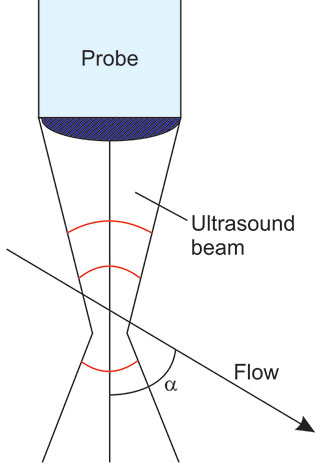
In medical applications, the Doppler effect is usually used by insonating the moving blood and assessment of the Doppler shift of ultrasound scattered on erythrocytes (Figure 1.2). Single erythrocytes reflect (retransmit) ultrasound in various directions, but the total back-scattered energy is sufficient for velocity assessment.
The general method of measurement consists of transmission of bundled ultrasound into the body at a general angle α to the flow. In this case, the following equation of Doppler shift is valid to sufficient approximation.
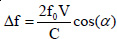

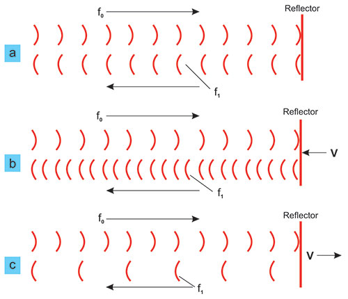
FIGURE 1.1: Illustration of the Doppler effect: change of frequency due to the movement of the reflector.

It has been demonstrated that for wave beams the Doppler shift is not exactly zero at α = 90°, but the shift is small and not used in the present commercial instrumentation (Figure 1.3). Thus, the plane wave approximation from the above equation is valid for the normal practice.3
From the above Doppler shift formula we can calculate the velocity, V with the help of the following equation:
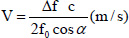
where c = ultrasound propagation speed; Δ f = Doppler shift; f0 = transmitted wave frequency; and α is the angle between the ultrasound beam and flow direction.
The flow in blood vessels depends on the quality of their walls and vessel dimensions. If the flow is laminar (when the walls are even and blood vessel is large enough) the flow profile is parabolic, that is, the velocity in the center is the fastest and slows down as we approach the walls. The law by which this changes is approximately a parabola (Figure 1.4). If there is an obstacle in the blood vessel (a plaque, a branching, etc.) the profile deviates from parabolic and can become turbulent. In any case, at any instance and at any cross section the blood flows at many different velocities at the same time, i.e. there is a full spectrum of flow velocities.
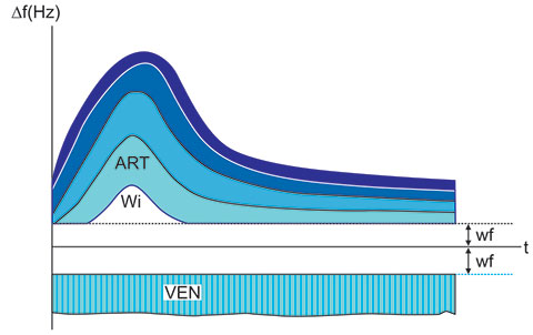
The results are usually shown as Doppler shift spectra in real-time according as in Figure 1.5.
The ordinate is the Doppler shift (Figures 1.5 and 1.6) and the abscissa is the running time. Doppler shift measured in Hz is proportional to flow velocity and if the angle α is known, one can put velocities onto the ordinate by using the equation for velocity calculation.
The upper spectrum (ART) has the typical shape of an arterial spectrum. It is pulsatile. The peripheral venous spectrum (VEN) in the lower part of Figure 1.5 is not pulsatile. Venous flow is not pulsatile in peripheral blood vessels but can be very pulsatile as the vessels approach the heart. Since the blood flows at each instance at different velocities, the spectra are generally filled-in. The lowest frequencies are cut off with special high-pass filters, the so-called, wall filters (wf). The filter was originally designed to eliminate the artifacts from moving blood vessel walls.
Apart from absolute velocity measurement, one can define relative indices, which are particularly useful for flow evaluation without known angle between the flow and ultrasound beam.
DOPPLER INDICES
Because of inherent difficulties in quantitatively evaluating blood flow, the blood flow velocity waveform has commonly been interpreted to distinguish patterns associated with high and low resistance in the distal vascular tree (Figure 1.6). Three indices are in common use, the systolic/diastolic ratio (S/D ratio), the pulsatility index (PI, also called the impedance index) and the resistance index (RI, also called the Pourcelot ratio).

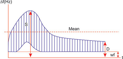
If we designate the peak systolic Doppler shift with S and the maximal diastolic Doppler shift with D, simple indices can be defined that roughly describe some properties of the spectra (Figure 1.6).
The S/D ratio is the simplest but it is irrelevant when diastolic velocities are absent and the ratio becomes infinite. Values above 8.0 are considered “extremely high”.
Definitions of RI and PI are as follows:

The RI is moderately complicated but has the appeal of approaching 1.00 when diastolic velocities are abnormally low and does, therefore, reflect the relative impairment of flow by high resistance. These indices are ratios, independent of the angle between the ultrasound beam and the insonated blood vessel and therefore not dependent on absolute measurement of true velocity.
The PI requires computer-assisted calculation of mean velocity, which still may be subject to very large experimental error. In a normal pregnancy, neither the S/D ratio nor PI is normally distributed across all gestational ages.
L Pourcelot and R Gossling initially derived the indices for their statistically demonstrated association with adverse clinical findings. However, the RI must not be considered independent of changes in physiologic variables, such as heart rate, cardiac contractility, blood pressure and the many other determinants of flow. This information does not depend on the measurement angle since all the parts of the spectrum change proportionally when angle α changes. However, as the angle approaches 90°, the measurement error increases drastically. In practice, it is the best compromise between the resolution of B mode image resolution and accuracy of Doppler spectroscopy is obtained at angles between 30° and 60°.
The three indices are highly correlated.2,3 There are intrinsic errors in all that have been quantified and lie between 10% and 20%. There may be advantages to the RI or PI where flow is markedly abnormal or in early pregnancy, when a very low end-diastolic velocity can be a normal finding.
INSTRUMENTATION FOR DOPPLER MEASUREMENTS
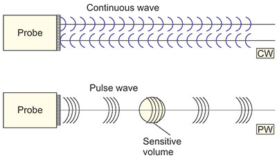
There are two basic technological methods for application of the Doppler effect in medicine (Figure 1.7). It is possible to transmit and receive ultrasound waves continuously with a probe that contains a transmission transducer and a reception transducer (continuous wave in Figure 1.7). Another possibility is to transmit in the form of pulses whose Doppler shift is measured after the time necessary for ultrasound to reach a defined depth in the body (pulse wave in Figure 1.7).
These two systems have different properties. The CW system has no depth resolution so that the measurement results of all flows along the line-of-sight add together and mix. On the other hand, this system measures well all (fast and slow) velocities. If there is only one blood vessel along the line-of-sight or one flow is dominant, the CW system is very good for practice.
If, however, one must measure the flow in a single blood vessel, the PW system can measure within a well-defined sensitive volume. The sensitive volume has a length that depends on the pulse length (in time) and a width that depends on the beam width (and focusing) (shown as sensitive volume in Figure 1.9). The disadvantage of such a pulse Doppler system is that it cannot measure high velocities deep in the body. The reason for this is that a PW system only occasionally looks at the flow so that it cannot convey all the information at an enough high throughput. The phenomenon can mathematically be described by the sampling theorem, which results in the so-called aliasing, i.e. reverse indication of flow that is too fast. The resulting artifact is shown in Figure 1.8. The top of the pulsatile spectrum (highest velocities) are shown as negative (reverse flow).

If the spectrum is simple like in Figure 1.8, the recognition of the aliasing artifact is easy. In complex spectra this can be hard. In such cases, it may be useful to have a combined PW and CW system or a HPRF system. The HPRF system has such a pulse rate that it violates the sampling theorem and thus yields mathematically ambiguous results. In the screen this is usually shown as multiple sampling volumes (spots, cursors). Such a system measures at multiple spots at a time. If the operator can recognize the spots with dominant flow or positions the cursors in such a way that only one of them hits flow, the system achieves a better performance for high velocity flow measurement.
Data Acquisition
The computerized generation of the flow velocity waveform is not a simple task. In addition to the modification of returned frequencies by scattering and tissue attenuation, a number of computer-based steps are required to eliminate low-frequency noise generated by tissues vibrating in response to the ultrasound beam and by nonultrasound-based movement of tissues.
Several processing mechanisms are used to modify and adjust the returned frequencies.
Both excessive low and high frequencies are filtered-out (band pass).
High-pass filtering (allowing only frequencies above a set minimum to be shown) removes unwanted low-frequency signals. Thus, interference from vessel wall vibration, or other tissue movement, is eliminated, but this mechanism will also remove low velocities representing low flow. High-pass filtering, therefore, is capable of erroneously suggesting absent flow in diastole. The operator can usually adjust this filter.
Sample volume (or “range gate”) limits the area (depth-wise) to be analyzed. In duplex scanning, the range gate is adjustable for length and for position. Range gating assumes a standard time interval between pulse emission and echo return that is based on the standard tissue transmit time from the depth set by the operator. The receiving gate is open only for the anticipated moment of echo return, thus restricting information received to what is “expected” from the area designated by the calipers on the screen. The sample volume should be larger than the vessel and positioned to span it completely if we wish to have complete data on the flow within the vessel. If it is set too large, extraneous signals may be included. If it is set much smaller than the blood vessel diameter, the resulting spectrum will be narrow (i.e. it will have a “window”) unless the flow is grossly turbulent.
These mechanisms, therefore, restrict the information that is returned and analyzed, in an effort to present an acceptable image. Such editing can discard some desirable data on (usually low) velocities.
Signal Processing
Since the pressure of the reflected ultrasound wave from blood is about a hundred times smaller that from the surrounding structures a substantially higher amplification is required. The data are then filtered and demodulated. Demodulation consists of comparing the transmitter carrier frequencies of the transducer's output, to reflected echoes. The so-called quadrature detector separates the demodulated signal in two channels, that is, flow toward the transducer is represented as positive Doppler shift and flow away from the transducer is represented as negative Doppler shift. The flow data are represented in real-time.
The spectral analysis is done with an algorithm called the fast Fourier transform, which makes a fast and approximate Fourier analysis of the signal.
Flow vs Velocity
The actual display is Doppler shift versus time. If the angle between the ultrasound beam and the flow is known, one can display velocity versus time. The actual measurement of the Doppler angle is often difficult. In some disciplines, the practice is to ignore the angle and speak about “velocities” (TCD, sometimes fetal echocardiography). The nature of the flow (pulsatile or steady, regular or turbulent, single or branching, parabolic or plug), impacts significantly on the frequencies returned. Thus, although volume blood flow can be calculated as the product of mean blood flow velocity and vessel area, this is fraught with variation in practical terms.6
The cross-sectional area of the vessel measured from the gray scale image is very susceptible to error. Additionally, the volume flow depends on the fourth power of the vessel diameter so that any measurement error is grossly amplified.4,5 Even the thickness of the distance measurement cursor plays a major role in measurement accuracy in blood vessels of a few millimeters in diameter.
Another major problem in measuring flow is the variation of blood velocity across the vessel cross section. Because the overall flow rate is the sum of the contributions made by the blood at every point on the cross section, it is necessary to average the velocity profile (mean blood flow velocity). Various approaches to this have been described. The calculation is different when the velocity profile is measured (with multigated pulsed Doppler) and averaged or if it is averaged using a large sample volume to encompass the whole vessel. Volume blood flow has been expressed as milliliters per minute. In fetal applications the result may be normalized to the fetal weight. Estimating the fetal weight by ultrasound measurement formulas is also error-prone. It is clear, to allow accurate or even vaguely useful volume flow measurement that Doppler interrogation must be limited to large vessels, with meticulous attention to methodology.
Figure 1.8 is an illustration of the aliasing effect on an arterial spectrum where the peak velocities have been too fast to measure with the particular pulse repetition frequency (PRF) of a pulsed Doppler system.
TWO DIMENSIONAL FLOW MEASUREMENT
2D Color Doppler Display
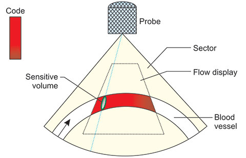
The flow can be shown in two dimensions (2D). In principle, comparison or subtraction of successive two-dimensional images can achieve this. Only echoes from moving structures stay in such images. The final result is a two-dimensional display of moving structures, mainly blood flowing through blood vessels.
The directions and speeds are color coded. Movements towards the probe are shown in different shades of one color, e.g. red and away from the probe in shades of another color, e.g. blue (Figure 1.9). The different shades signify relative velocity. One must always bear in mind that this system shows the component of velocity projected onto the probing ultrasound beam. This makes the display semi-quantitative. One can display the multiple Doppler shift measurement variance. In the red-blue combination code, the variance is usually shown in green. The larger the measurement variance—the more green. This gives an indication of turbulence. Flow at 90° to the ultrasound beam are not shown (in the image they are shown black, i.e. as if it were not there). The color code is arbitrary and in the majority of machines can be chosen from a number of different possibilities. Since the 2D, color Doppler is semi-quantitative, it is as a rule combined with a PW Doppler spectrometer. The 2D display helps in fast finding of the points where we wish to analyze the flow by spectrometry. In this way, the 2D system reduces the duration of Doppler examinations. Sometimes, however, the 2D map is characteristic enough to help with the diagnosis. The limitations of the method are equal to the pulse Doppler technique and so we got the, now ubiquitous “Color Doppler”. As with any new method, the first amazement yielded its place to systematic and often controversial, but always tedious evaluation in clinical medicine. Since many of the most feared illnesses develop on a long time scale, the method is still under scrutiny but is already accepted as a useful tool.

A particular form of 2D flow mapping is the, so-called, Power Doppler (Figure 1.10).
Power Doppler Ultrasound
The shortcomings of the two-dimensional directional Doppler (“color Doppler”) are many. Above all, the sensitivity to direction is a mixed blessing. It does give the much-valued information about the direction of flow, but suffers from not-very-high sensitivity and direction artifacts. Now, in many cases the directional information, if very valuable, like in echocardiography. However, there are many instances when the only relevant question is “Where are the blood vessels?” or “How many blood vessels are there?” or “What is the perfusion of this area?”.7
The direction may be of little importance or determinable with a built-in Doppler spectrometer. Basically color Doppler yields that information. However, it is not uncommon to find a clear Doppler spectrum signal from an area that is completely without any color signal or where (if we are lucky) the color appears occasionally. The reason for this is that the directional information is evaluated from a number of subsequent frames and ambiguous and low signals average out to zero.
All these considerations led the instrumentation researchers to take a step backward and develop a two-dimensional system, which just detects and displays movement; any movement, in two dimensions. The result is an instrument, which displays areas with moving structures in color. The color means that there is flow in the area and the brightness of the color qualitatively indicates the quantity of moving erythrocytes.6
Every normal color Doppler system has the basic capability for “power Doppler” or “Doppler Angio”. Actually the power Doppler is a mode of operation in which any signal, which shows a Doppler shift (change in frequency) is tagged with color. So the direction becomes irrelevant. Unlike color Doppler where a symmetrical turbulence shows a poor signal, in power Doppler, the signal will be as strong as any. The reason for this is that when directional information is displayed, the zero mean velocity is not displayed, while in the case when the total reflection from any moving structure is displayed a turbulent flow is as indicative as any.
The decision as to what is flow and what is not is taken by looking at the frequency spectra and high enough frequency shifts are considered to represent blood flow. The color-coding is made proportional in brightness to the total power of reflected ultrasound from moving structures. Structures which do not move or move slowly are not color-coded.
The displayed color indicates the quantity of moving blood, but not the volume flow of blood per unit time. Actually the virtue of this display mode is that it shows about equally fast and slow flow so that we can get a feeling of the general blood perfusion in some area. However, if actual blood velocity or volume per unit time is of any interest, we must revert to other display and measurement modes.
The returned signal depends, in addition, on the attenuation of ultrasound in the intervening tissue. This means that the flow in deeper blood vessels or the flow in the same blood vessel that changes the depth will be shown with different brightness, depending on the depth. The density of the moving blood cells depends on the concentration of blood cells and local flow situation. The sampling volume depends on the length of ultrasound pulse and beam width. If the sampling volume is larger than the blood vessel, the average number of red blood cells in it will be smaller and the returned signal will be thus relatively weaker, showing a dimmer color on the display.
BASIC LIMITATIONS OF DOPPLER EXAMINATIONS
In Doppler measurements one encounters problems of accuracy, precision and artifacts like in any measurement and imaging method. The peculiarities of this method are as follows:
Accuracy
- Doppler spectrometry operates adequately for angles between ultrasound beam and flow less than 60°. The theoretical measurement error tends asymptotically towards infinity when the angle approaches 90°. The raw result of the measurement is a spectrum, which illustrates well the general behavior, but has the data on velocity hidden by an additional unknown factor—the angle. However, even with the angle a known, data like mean velocity can be calculated only by way of a fairly complicated numerical integral of the weighted spectrum. The automaton, which picks up the respective weights of single velocities within the spectrum at each instant operates fairly autonomously, usually without intervention of the operator. The intervention by way of changing measurement sensitivity can change the result of the calculation. One must continuously bear 8in mind that we measure Doppler shift only, while the rest of the data is derived from it. The accuracy of assessment of the Doppler shift really depends on the knowledge and control of the frequency content of the ultrasound pulses. This is often not well controlled. An exception is operation with CW Doppler systems where the measurement can be made more accurate.
- Color Doppler itself is not designed as an accurate measurement method, but mainly a semiquantitative guiding method for Doppler shift spectroscopy. In spite of this, the significance of different colors must be known and in particular one must carefully adjust the base-line shift since this can essentially change the velocity-color map.There exists, however, a possibility to extract the accurate data on the Doppler shift by using a cursor, which helps in reading the frequency shift from the computer memory.Fourier power spectra, where available, give quantitative data but are often not well understood. This spectrum is not a real-time spectrum but a graph with Doppler shift on the abscissa and the energy in frequency range on the ordinate. Its width and symmetry properties contain ample information about the nature of the flow (which is harder to read from a usual real-time spectrum). One should not confuse this power spectrum with the “Power Doppler”.
- Power Doppler display method has a slightly better geometrical accuracy in showing the blood vessel lumen than the normal “color Doppler”. This happens at the cost of image repetition rate.
Precision
- The quantitative functional dependence of the velocity measurement error on the knowledge of the angle α is known. However, the usual method of measurement of the angle is very crude and thus one should try to avoid using absolute values whenever possible.
- Since the color map scale is virtually continuous there is only marginal accuracy in the judgment of the velocity by way of color assessment. However, the variance map, although not accurately assessable gives a very useful clue as to where one ought to do spectroscopic measurements. Again, the Fourier power spectra capability enables a precise variance calculation and the Power Doppler modality increases observation sensitivity at the cost of loosing directional information.
CONTRAST MEDIA
The energy reflected (scattered) back from the erythrocytes is about 10,000 times smaller than the energy reflected from the blood vessel walls. This presents serious technological sensitivity problems. One of the possibilities to increase the sensitivity is to use contrast particles as scatterers instead of erythrocytes. The contrast media are basically composed of bubbles of gas or liquid enclosed in thin nontoxic, usually organic membranes. Such bubbles are of well defined size and stable enough to stay in the circulation long enough to make the required Doppler measurements before dissolving and disappearing from the circulation. They reflect ultrasound much better than erythrocytes proper and thus alleviate much of the sensitivity problems.
In addition to helping Doppler measurements, the contrast media can modify and enhance normal echographic images. A concentrated effort in research is underway to make various parameters of the contrast media more specific, e.g. resonant at specific frequencies or with biologically active membranes.
Artifacts
Several artifacts are encountered in Doppler ultrasound.7–12 These are incorrect presentation of Doppler flow information (Table 1.1). The most common of these is aliasing. However, others occur, including range ambiguity, spectrum mirror image, location mirror image, speckle and electromagnetic interference.
Aliasing
There is an upper limit to Doppler shift that can be detected by pulsed instruments. If the Doppler shift frequency exceeds one half the pulse repetition frequency, aliasing occurs and improper Doppler shift information (wrong direction and wrong value) results. An analogous optical form of aliasing occurs in motion pictures when wagon wheels appear to rotate in reverse direction (This happens here because the number of pictures per second is insufficient to correctly show the rotation speed). Higher pulse repetition frequencies permit higher Doppler shifts to be detected but also increase the chance of the range ambiguity artifact. Continuous-wave Doppler instruments do not have this limitation but neither do they provide depth resolution.9
Aliasing can be eliminated by increasing pulse repetition frequency, increasing Doppler angle (which decreases the Doppler shift for a given flow), or by baseline shifting. The latter is an electronic “cut and paste” technique that moves the misplaced aliasing peaks over to their proper location. It is a successful technique as long as there are no legitimate Doppler shifts in the region of the aliasing. If there are, they will get moved over to an inappropriate location along with the aliasing peaks. Other approaches to eliminating aliasing include changing to a lower frequency Doppler transducer or changing to a continuous-wave instrument, which is often built-in into specialized cardiologic units. Aliasing can occur in a pulse system since it is a sampling system, which cannot yield a correct result unless it samples often enough, that is, twice the highest Doppler shift frequency. This is called the Nyquist limit (of the sampling theorem).
Increasing the pulse repetition frequency can reduce the aliasing problem. However, this can cause localization ambiguity. This occurs when a pulse is emitted before all the echoes from the previous pulse have returned. When this happens, early echoes from the last pulse are simultaneously received with late echoes from the previous pulse. This causes difficulty with the ranging process. In effect, multiple gates or sample volumes are operating at different depths. Multiple sample gates are shown on the display to indicate this condition. Range ambiguity in color-flow Doppler, as in sonography, places echoes (color Doppler shifts in this case) that have come from deep locations after a subsequent pulse was emitted in shallow locations where they do not belong. As already said, the HPRF systems intentionally introduce this ambiguity for spectrometry, requiring sound judgment by the operator as to whether the results are correct or not. Comparison of different Doppler instruments is given in Table 1.2.
The mirror image artifact can also occur with Doppler systems. This means that an image of a vessel and a source of Doppler shifted echoes can be duplicated on the opposite side of a strong reflector (such as a bone). The duplicated vessel containing flow could be misinterpreted as an additional vessel. It will have a spectrum similar to that for the real vessel. A mirror image of a Doppler spectrum can appear on the opposite side of the baseline when, indeed, flow is unidirectional and should appear only on one side of the baseline. This is an electronic duplication of the spectral information. It can occur when receiver gain is set too high (causing overloading in the receiver and cross talk between the two flow channels) or with low gain (where the receiver has difficulty determining the sign of the Doppler shift). It can also occur when Doppler angle is near 90º. Here the duplication is usually legitimate. This is because beams are focused and not cylindrical in shape. Thus, portions of the beam can experience flow toward while other portions can experience flow away. An additional possibility is to fit a bend of a small blood vessel in the same sample volume, which then yields opposite flows in the two parts of the “hook” as opposite, nearly symmetrical spectra.
| |||||||||||||||||||||||||||||||||
Occasionally, a spectral trace can show one or more straight lines adjacent to and parallel to the baseline, often on both sides.
This is due to any electrical noise operating at multiples or whole fractions of the monitor image repetition, including 50 Hz interference from power lines or power supply. It can make determination of low or absent diastolic flow difficult. Electromagnetic interference from power lines and nearby equipment can also cloud the spectral display with lines or “snow”. Improper pulse repetition frequency (PRF) settings can ultimately cause erroneous diagnosis of an absent diastolic blood flow.
In Figure 1.5, “WI” indicates the “window”, an empty space in the real-time spectrum. Strictly speaking, this space ought never be empty, but in the case of parabolic flow and somewhat reduced sensitivity, the space will not fill in with measurement results. This logic applies, if the sensitive volume takes up the whole blood vessel cross section. However, if we reduce the sensitive volume so as to take up only a small part of the blood vessel, a “window” will appear even at fairly irregular flows. This does not influence much the assessment of RI and PI, but disturbs our assessment of the turbulence. Very turbulent flow will show at the same time positive (towards probe) and negative (away from probe) flow spectrum. However, a similar spectrum appearance can be expected if we put the measurement angle near 90º. Therefore, we must always interpret the cause of the apparent synchronous flow in opposite directions.
Inadvertent change of the wall filter can cut off the diastolic part of arterial Doppler spectrum and lead to wrong clinical diagnosis.
How to Reduce Problems
- Use the sensitivity with caution (use as a low sensitivity as practical)
- Start examination with the standard symmetrical color map and then gradually change it to nonsymmetrical types, if needed.
- Be aware of the depth and increased aliasing probability at deeper structures and higher velocities.
- Use all the three modes (B mode, spectrum, color) for survey, but use single modality to obtain the best quality of each of them.
Acknowledgment
In writing this chapter some materials provided by Ivica Zalud, MD, PhD have been used and this is kindly acknowledged.
REFERENCES
- Censor D, Newhouse VL, Vontz T, et al. Theory of ultrasound Doppler-spectra velocimetry for arbitrary beam and flow configurations. IEEE Trans Biomed Eng 1988; 35 (9): 740-51.
- Burns PN. Principles of Doppler and color flow. Radiol Med 1993; 85: 3-16.
- Taylor KJ and Holland S. Doppler ultrasound. Part I. Basic principles, instrumentation, and pitfalls. Radiology 1990; 174: 297-307.
- Mitchell DG. Color Doppler imaging: principles, limitations, and artifacts. Radiology 1990; 177 (1): 1-10.
- Kremkau FW. Doppler color imaging. Principles and instrumentation. Clin Diagn Ultrasound 1992; 27: 7-60.
- Chen JF, Fowlkes JB, Carson PL, et al. Autocorrelation of integrated power Doppler signals and its application. Ultrasound Med Biol 1996; 22 (8): 1053-7.
- Zalud I and Kurjak A. Artifacts and pitfalls. In: Kurjak A (Ed). Transvaginal color Doppler, (2nd Edn), London-New York: Parthenon Publishing 1994; 353-8.
- Derchi LE, Giannoni M, Crespi G, et al. Artifacts in echo-Doppler and color-Doppler. Radiol Med 1992; 83: 340-52.
- Jaffe R. Color Doppler imaging: A new interpretation of the Doppler effect. In: Jaffe R and Warsof SL (Eds). Color Doppler imaging in obstetrics and gynecology. McGraw-Hill New York: 1992; 17-34.
- Winkler P, Helmke K, Mahl M. Major pitfalls in Doppler investigations. Part II. Low flow velocities and colour Doppler applications. Pediatr Radiol 1990; 20 (5): 304-10.
- Suchet IB. Colour-flow Doppler artifacts in anechoic soft-tissue masses of infants. Can Assoc Radiol J 1994; 45 (3): 201-3.
- Pozniak MA, Zagzebski JA, Scanlan KA. Spectral and color Doppler artifacts. Radiographics 1992; 12 (1): 35-44.
- Maulik D. Biosafety of diagnostic Doppler ultrasonography. In: Maulik D (Ed). Doppler ultrasound in obstetrics and gynecology. Springer New York: 1997; 88-106.
- Duck F, Zauhar G. Report on experiments by Starrit H, Zauhar G and Duck F in Bath, Autumn 1996.