

Chapter Outline
- □ Getting Started
- □ Physics of Transducer Choice
- □ Resolution
- □ How and Why Knobs that Should be Used Often, Should be Used
- □ Doppler Studies
- □ 3D and 4D Ultrasound
- □ Safety of Ultrasound
Introduction
While a basic knowledge of the principles of physics of ultrasound for the everyday practice of ultrasound is essential, a deep understanding may not be necessary. This is equally relevant to ultrasound in subfertility as well. What is more pertinent is a working knowledge of how the machine acquires, processes and displays an image, and how the knobs and software improve the image. The aim is to obtain an image that quickly and reliably helps to answer the questions that are sought from the examination.
Getting Started
In order to rapidly obtain optimal images on a daily basis, a three-step training strategy is what is often useful. This requires no knowledge or understanding of physics or the principles of ultrasound and is an empirical approach to a quick start. The first step is an all-important and efficient shortcut of a hands-on demonstration of each knob and menu of the unit by an applications expert from the manufacturer. This should be followed by a hands-on routine on the patient with the applications expert standing by for a few days. The third step is working with the unit independently. As a final follow-up, it is wise, efficient and inexpensive to recall the applications expert for 1 day on every 3 weeks or so for a few months, so that the technology in the unit is then optimally utilized. Follow-up exposure at workshops that demonstrate newer equipment and techniques by experts is useful for refining technique on an ongoing basis and learning newer applications. At this stage, a working knowledge of applied physics and applied mathematics becomes indispensable.
This chapter is a practical treatise of applied physics in the perspective of obtaining an optimal image. Pure physics has been dispensed with, since it would occupy unnecessary space in this book!
Physics of Transducer Choice
The choice of transducers in evaluating subfertile and indeed, all gynecological patients is based on the understanding of two equations in physics. The first is the relationship of frequency (f) and wavelength (λ). Velocity (ν) is a product of wavelength and frequency (ν = λf). The second equation relates to ultrasound beam geometry. The depth (d) at which the transition of the beam takes place from the near field to the far field is given by the equation d = r2/λ, where r is the diameter of the circular transducer. Information from these relationships yields guidelines for tailoring transducer use.
The velocity with which a sound wave makes its way through any material is dependent on the density of the medium and is 330 m/s in air, 1,480 m/s in water, 1,589 m/s 2in muscle and 3,500 m/s in bone.1 Ultrasound machines are now standardized and calibrated to use 1,540 m/s as the speed of sound in human tissue. Since the velocity is a product of wavelength and frequency (ν = λf), the higher the frequency the shorter the wavelength. Frequency refers to the degree of highness or lowness of a tone. The loudness of a tone is referred to as intensity.
Low-frequency sound, such as the human voice, spread all over a room. High-frequency sound behaves like light and moves like a beam along a straight line. High-frequency ultrasound moves through tissue as a narrow beam and can be focused by acoustic lenses. This is possible in the nearer relatively narrow part of the beam. The depth equation (d = r2λ) implies that the wider the transducer face and the longer the wavelength (i.e. low frequency) the greater the depth. Resolution, however, depends on frequency, and therefore, the higher the frequency the better the resolution.
The vast majority of scans in fertility patients are transvaginal scans. Since the transducer is closer to the region of interest than with transabdominal scans, a higher transducer frequency can be used. This greatly enhances resolution. Currently available transducers employ frequencies of up to 12 MHz, and the difference in resolution is remarkable (Figs 1A and B). The trade-off with higher frequencies is of course, depth penetration of the beam, and these higher frequency transducers have a limited resolution beyond a certain distance from the transducer. This limitation can be overcome by using a multifrequency transducer. Console keys permit a choice of low, middle and high frequencies with the same transducer, enabling a great combination of resolution and depth. Transabdominal transducers have an advantage of a more panoramic field of view and a greater depth of penetration. These are therefore useful for identifying extraovarian adnexal structures and ovaries located at the pelvic brim. They are also indispensable for the assessment of associated abdominal lymph node disease, the suprarenal glands, kidneys, liver, abdominal peritoneal disease and the pleura.
Transvaginal transducers are either mechanical or electronic array transducers. Mechanical transducers have one or more crystals that rotate or oscillate. Electronic transducers either have an array of crystals that are fired sequentially (phased array) or a set of crystals shaped to produce the sector image.2 A large number of variations on these three types are commercially available and the user is warned to sift through the hyperbole and mystique of pseudophysics in making a choice! In general mechanical transducers are less expensive. They have a wide field of view but have poorer resolution in the near field. Focal zones are fixed. Electronic array transducers cost more but have the advantage of good near field resolution and multiple focal zones.
Resolution
Technically, resolution refers to the ability of the ultrasound unit to differentiate two different adjacent structures as two discrete different structures and not fuse them into a single structure. High resolution refers to a very short distance between these two structures, and low resolution refers to a larger distance between these structures.
Axial resolution refers to the resolution along the path of the beam and is the most discerning resolution. This is also termed as the radial resolution or the range resolution. The shorter the pulse, i.e. the higher the frequency, the better the axial resolution.
Lateral resolution refers to resolution in the plane perpendicular to the plane of the beam. This is also called the azimuth plane. Beam quality and the size of side lobes determine lateral resolution. Side lobes are like skirts around the main lobe. “Main lobe” refers to the thin, round, useful portion of the ultrasound beam.
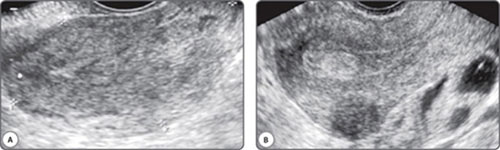

Figs 1A and B: Images from the same patient using a (A) 5 Mhz and a (B) 12 Mhz transducer frequency. The inhomogeneous endometrium translates into an echogenic polyp. The indistinct posterior uterine wall on a higher frequency reveals an intramural fibroid. Thick-walled fluid loculi are evident posterior to the uterus on a high frequency study
When such a beam passes through tissue and is reflected back, structures in the side lobe zone are wrongly assigned to the main beam. These falsify and degrade the image. Lateral resolution can be improved by focusing the ultrasound beam. This is achieved by complex technology. From a practical viewpoint, arrows along the margin of the image indicate focused areas and these can be manually set to enhance the axial resolution at the depth of interest. This is a simple and extremely useful step in imaging but is largely neglected by most operators.
Axial resolution has a direct bearing on measurements. Since axial resolution is superior to lateral resolution, measurements are more accurate in the axial direction.
Elevation plane resolution refers to resolution in the slice thickness perpendicular to the axial plane. Good elevation plane resolution prevents superimposition of solid echoes over cystic areas in the slice thickness. This aspect of resolution is not electronically enhanceable and is achieved by a fixed acoustic lens. Limitations in this plane can be overcome only by operator's knowledge, skill and vigilance.
How and Why Knobs that Should be Used Often, Should be Used
Depth, Magnification and Zoom
Depth refers to the depth of tissues on display. It is wise to commence with a deeper region of interest to ensure that deeply located lesions are not missed. The depth is then reduced to a level that includes the region of interest. Typically, the depth should be adjusted so that the main area of interest ultimately occupies two-thirds of the screen.3 Reducing depth increases magnification in the near field and this improves resolution. All available pixels are used to form the image, and the image therefore improves.4 When the depth is too large it takes much longer for the transducer to receive echoes that return from deeper structures. This reduces the frame rate adversely. The zoom function allows magnification of one area on the monitor.3 The image appears larger. The resolution of the magnified area does not change. Zoom allows a better study of small areas of interest. Beyond a point in zoom mode, the pixels become too few and the image becomes grainy. The structure to be assessed in detail should, therefore, be imaged at as shallow a depth as possible.
Zoom selects a square area that is sized in real time before it is activated. Depth should be adjusted before zoom is selected.
Gain
Adjusting gain alters how the transducer perceives returning echoes. Increasing the gain brightens the display of the returning echo information. Gain may be adjusted for the entire image (overall gain), or at depth, known as time-gain compensation (TGC).3 Excessive gain makes the image too bright, and too little gain makes it dark (Figs 2A and B). Excessive gain can make the picture bright with noise. This can obscure fluid echoes (Figs 3A and B). Too little gain may create fluid echoes where no fluid exists (Figs 4A and B). Many currently available medium and high-end units now have a one-touch image optimization button that works automatically to fix the gain in an image.
Power Level
Power and Gain are not the same. Power level refers to the amount of energy produced by the transducer.4 Gain amplifies returning waves. Increasing the power helps to image deeper structures. It may, however, produce secondary vibrations in tissues. This can produce ring-down artefacts (Fig. 5). Some sound energy may bounce back and forth within a cyst resulting in reverberation artefacts (Fig. 6).

Figs 2A and B: Excessive gain obscures textural detail. There is excessive gain in the image on the left (A) and the texture and margins of the endometrium are indistinct. The image on the right (B) has optimal gain. The triple layered proliferative phase morphology is distinct and no focal lesion is evident
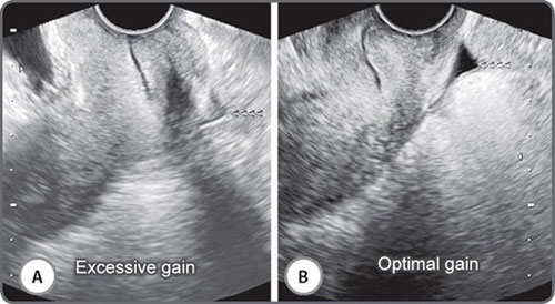
Figs 3A and B: Excessive gain can obscure fluid echoes. The image on the right (B) was obtained at optimal gain settings and shows a small quantity of free fluid (<<<<) in the pouch of Douglas. The image on the left (A) was obtained at high gain settings and the fluid (<<<<) is largely obscured

Figs 4A and B: Inadequate gain can “create” fluid where none exists. In the image on the left (A); a large fluid collection is evident in the right adnexa. Increasing the gain [right (B)] reveals an ovary with three antral follicles

Fig. 5: Increasing the power in order to image deeper structures may produce secondary vibrations in tissues. This can produce ring-down artefacts
Power that is too low produces a faint image.4 A weak signal gets mixed up with inherent noise in any equipment, and the result is a degraded image called snow4 (Figs 7A and B). Power should, therefore, be adjusted to ensure a balance between snow and artefacts.
Tissue Harmonic Imaging
While conventional ultrasound uses the same frequency bandwidth for both the transmitted and received signals, tissue harmonic imaging (THI) uses a low frequency for transmitted signal and a high frequency for the received signal. When echoes return after being reflected, they do so not only at the basic frequency but also at multiples of the basic frequency. These higher frequency waves experience less attenuation, less scatter and less side lobe artefact and may generate clearer images, particularly at the interface between fluid and tissue. The trade-off is a slightly longer processing time. This is now routinely available on most ultrasound machines.
Dynamic Range
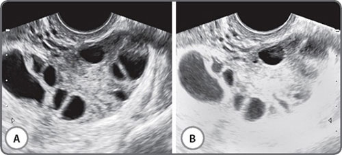
A clear cyst is best assessed with a minimum of gray levels. A wider range of grays better assesses solid lesions. Dynamic range permits this variation of gray scale (Figs 8A and B). Dynamic range is the range in acoustic power between the faintest and strongest signals. Dynamic range controls the image contrast with increasing the dynamic range produces a grayer image.
Focal Zones
While doing ultrasound scan, one should constantly check the position of focal zone/s to ensure that they are at the depth of interest.
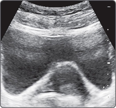
Fig. 6: Reverberation artefact. High-level echoes are seen in the anterior extent of the urinary bladder. These may obscure solid lesions and also render an entirely fluid lesion echogenic
Figs 7A and B: Inadequate power and excessive gain combine to create noise called snow (B). This creates medium sized high level echoes which obscure margins and fluid densities in the region of interest when comparing with the image obtained with optimum power and gain (A)

Figs 8A and B: Solid organs and lesions are best studied by a wide dynamic range setting. The image on the left was done at fluid level settings and failed to reveal an 8 mm echogenic polyp in the endometrium. The image on the right was optimized with a wide dynamic range and clearly (<<<<<<<) shows an echogenic endometrial polyp
Multiple focal zones, which create a long narrow beam, can be used to maximize lateral resolution over depth with the overall image quality will be improved throughout a static image. But it is best to minimize the number of focal zones, when assessing moving structures as it may take more time to form a scan line and result in frame rate being reduced making the images disjointed.
Presets
Most current machines have settings that will adjust an image based on the anatomy being scanned. These presets are programmed to optimize images based on certain gain and power settings, focal zones, frame rates and other settings.3 It is imperative that the applications expert checks factory set presets.
Doppler Studies
The term “Doppler” is loosely used to indicate blood flow information. It is based on the Doppler effect wherein the returning frequency of waves is altered by the movement of a target. The moving target is Red Blood Cells in the blood vessels in the region of interest. The returning signal is mapped in two ways.5 A map of the vessels can be obtained which can be superimposed on the gray scale image. This is known as color flow mapping. This indicates direction and velocity of flow. The other method of mapping is known as the Doppler spectrum. This consists of a graph showing flow characteristics as a waveform (Fig. 9). These can then be quantified as velocities, ratios and indices. The Doppler spectrum has an equivalent simultaneous audio signal as well which one learns to assess and analyze with increasing experience.6
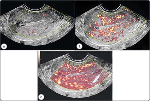
Power Doppler is a newer form of flow imaging. It uses amplitude of scatter rather than a frequency shift to make a map of tissue flow. It is by its inherent nature far more sensitive to slow flow and therefore extremely useful in evaluating cyclical and pathological changes in the female pelvis. Recent technical advances have made power Doppler directionality available as well.
Doppler requires fine-tuning of sets as much as does gray scale.
Pulse Repetition Frequency or Scale
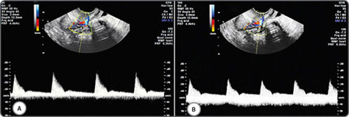
Adjusting the pulse repetition frequency (PRF) alters the sensitivity of Doppler for flow velocity (Figs 10A to C). A lower PRF will result in a lower scale, more sensitive for slower flows, but may cause aliasing artefacts.3 PRF should be ideally kept low when assessing vessels with low velocity blood flow (eg: ovarian stromal arteries) and be kept high when assessing vessels with high velocity blood flow (eg: uterine arteries).


Figs 10A to C: Doppler PRF settings: PRF settings should be kept low for vessels with low velocity blood flow and high for vessels with high velocity blood flow. This figure demonstrates the effect of PRF on velocity wave form on an ovarian stromal vessel. PRF is kept low (A), optimum (B) and high (C)
Doppler Gain
Similar to the basic B-mode or two-dimensional image, gain may be adjusted for Doppler. Increasing Doppler gain will amplify returning signals, resulting in more color or a stronger spectral signal (Figs 11A to C and Figs 12A to C). As in B-mode imaging, too much gain will result in noise and artifact.7 Doppler gain should be set so that the vessel lumen is filled with color but there is no spill outside.
Baseline
Doppler can display flow either toward or away from the probe. Typically for color or spectral Doppler, the “zero” is in the center of the scale (or Y-axis). If you want to look only at the positive or negative flow, you can adjust the baseline up or down.
Wall Motion Filter
Filter allows adjustment of the signal so that lower velocities up to a certain number will not be displayed. A higher filter will reduce artifact but may limit visualization of lower flow (Figs 13 and 14).3
Probe Angle
When red blood cells move perpendicular to the ultrasound beam, the transducer fails to detect them.4 Most machines, fortunately, will detect signals with even a minimal change beyond the perpendicular plane. When a vessel is anticipated to have slow flow, it should be imaged more vertically to the transducer.
Color Box Size
Large box sizes result in large amounts of data for processing. This slows the rate at which images are generated. Even if the frame rate is increased, this delay in generating an image is not easily overcome. Until large computers get incorporated into machines, and this will happen only if computers get cheaper, small color boxes should be used.4
Sample Volume Size and Position
The precise location of sample volume may affect the appearance of the Doppler spectrum and therefore may affect the results of spectral Doppler measurements. The relationship between the size of the sampling box applied with pulsed-wave Doppler and the size of the vessel is another important consideration (Fig. 15). The average flow velocity within the center of a small vessel may be double to that of the average velocity across its full width due to turbulence near the vessel wall.
Figs 11A to C: Doppler gain (Power Doppler): Increasing gain will amplify the returning signal resulting stronger Doppler signal. The gain is kept low (A), optimum (B) and high (C). Too much gain in (C) results in artefact signals

Figs 12A to C: Doppler gain (Pulse wave): Increasing gain will amplify the returning signal resulting stronger Doppler signal. The gain is kept low (A), optimum (B) and high (C)

Figs 13A and B: Wall motion filter (Power Doppler): A higher filter setting (A) limits artifacts, but limits visualisation of lower flows, when compared with optimal setting (B)

Figs 14A and B: Wall motion filter (pulse wave Doppler): A higher filter setting (A) can affect pulse wave forms in comparison with optimal setting (B)
Figs 15A and B: Doppler sample volume (Doppler gate) size and location: The width of the Doppler gate is kept 2 mm (A) and 3 mm (B). In figure (B), the Doppler gate is wider than the diameter of the artery and is placed partly over an adjascent vein and therefore picking up both arterial and venous flow
It follows therefore that too small a sample box placed centrally over a vessel may over-estimate the true flow. Whilst the diameter of the ascending uterine artery ranges from 2 to 5 mm in the non-pregnant patient, the spiral arteries at the level of the endometrium measure 1 to 2 mm in diameter. The diameter of the ovarian stromal vessels are also around 1 to 2 mm. This leaves little room for placement error considering 9the smallest volume box usually starting at 1 mm. The width of the volume box (Doppler gate) should be adjusted to the inner diameter of the vessels to be evaluated.
Doppler Angle (Angle of Insonation)
The angle of insonation between the Doppler beam and the direction of vessel is generally calculated by the observer who rotates a line so that it lies parallel to the direction of blood flow (Figs 16A to C). A 5° error in the orientation of this line leads to an error in the velocity measurement of <2.0%, but this increases to 5.4% if the real angle is 30° and 12% when it is 60°. In this respect, the most accurate velocity measurements are made when the angle of insonation is as close to zero as possible but this is not always possible as it is dependent upon the position and direction of the blood vessel being studied.
3D and 4D Ultrasound
In this era of rapidly evolving technology, three-dimensional (3D) and real-time three-dimensional (4D) ultrasound are emerging as necessary tools in the assessment of the pelvic viscera. As for other anatomical regions, freehand or automated devices may be used to acquire volume data for 3D evaluation of pelvic organs. In the freehand method, the transducer is manually moved through the region of interest and a position sensor registers the slice in space and time, or alternatively, image based software may be built into the 3D package. The freehand method may be used on-line where the ultrasound unit manages all functions, or off-line where the analog video output is fed into a workstation. The transducer and attachments in the free-hand system are bulky and awkward to use particularly in the vagina. Most units currently in vogue are automated 3D probes. These are unit specific, more accurate and easy to use. When these units are employed, an area of interest is chosen in the real-time 2D image, and the size and depth are outlined. A speed of acquisition is then selected and the acquisition activated. The transducer elements automatically sweep through the volume box chosen. The slower the speed of acquisition the higher the resolution. Resolution is highest in the plane of acquisition. The closer the plane of acquisition to the plane of study the better the resolution. The machine automatically receives and stores data from the region of interest and displays it in an orthogonal format.

Figs 16A to C: Doppler angle (angle of insonation): The angle of insonaton between the Doppler beam and the direction of vessel can affect the velocity measurements. At angles of insonation of 22° (A), 30° (B) and 68° (C), respectively, peak systolic velocity (PS) measurements from the same vessel were 21.33 cm/s, 27.11 cm/s and 56.87 cm/s
Images may then be rendered by various algorithms which rely on the difference between acoustic impedances at tissue interfaces and have been variably named by various manufacturers. In conventional ultrasound, the endometrium is visualized as a variably thick, linear or ovoid structure in longitudinal, transverse and oblique plane. The shape of the cavity is difficult to assess, as is the coronal plane. With 3D, the entire extent of the endometrium can be shown, including the corpus, fundus, cervix and cornual areas.8 Coronal, sagittal and transverse planes can be simultaneously displayed to permit more exhaustive viewing (Fig. 17).
The images may be automatically zoomed in or out. Once acquired, the volume data can be reviewed by first rotating the planes to obtain standard anatomic orientations and then scrolling through the entire data to locate and characterize lesions, both focal and diffuse. Multiplanar orthogonal viewing offers virtually unlimited numbers of planes, and time constraints should not impede the endeavor to obtain information. In fact, the additional time spent on a 3D gynecologic scan is far less than on 3D obstetric scan because this time is spent not so much on data acquisition but in exploring the data obtained. The time factor would, of course, depend on the complexity of a case and on operator expertise. In experienced hands the exercise takes no more than 3–10 minutes. Once identified in any one plane, the lesion can be marked by a center point, and this center point is automatically displayed in all three orthogonal planes. All or part of the studied volume can be automatically rendered and displayed as a single image or along with the orthogonal planes. The evaluation is enhanced by using volume measurements, niche mode studies, power Doppler studies and a retrospective review of stored data. Unlike obstetric 3D, surface rendering is infrequently required in gynecologic 3D studies except in saline infusion sonohysterography where it often adds diagnostic information. The entire acquired data can be transmitted electronically to obtain second opinions, facilitate remote conferencing with experts, and can be efficiently stored for review and recall.
The sagittal plane is selected for volume measurements and the other two planes for ensuring that the entire pathology is included in the measured area. Surface rendering permits contoural evaluation. Niche mode studies permit a virtual tour of the entire lesion and surrounding tissue along with evaluation of vascular morphology. 3D power Doppler permits an unsurpassed view of vascularity and permits quantification of neovascularization. 3D saline infusion sonohysterography enhances the sensitivity in select situations. Real-time 3D (4D) is useful in saline infusion sonohysterography for storing data sets, excluding the need for re-instillation, permitting multiplanar analysis and allowing magnification of stored data during re-evaluation.
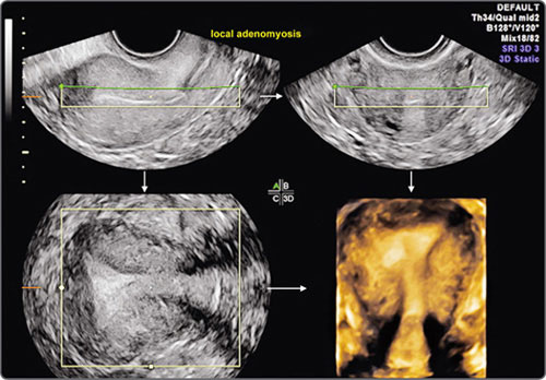
Fig. 17: 3D multiplanar view of an uterus showing longitudinal plane (upper left), transverse plane (upper right), coronal plane (lower left) and rendered view of transverse plane (lower right)
In patients who have not been sexually active, 3D data acquisition via the rectum, using an intracavitary transducer, can greatly enhance delineation of pelvic lesions and developmental abnormalities when compared to transabdominal 3D studies.
Three-dimensional data is basically a sum total of 2D data sets, and, as a logical consequence, a 3D study does not replace a 2D study. It, in fact, extends the wealth of information obtainable from an ultrasound scan. Principles of 3D ultrasound and its application in subfertility is further detailed in chapter 13.
Safety of Ultrasound
The Bioeffects Committee of the American Institute of Ultrasound in Medicine has repeatedly established based on the available evidence that there are no confirmed biologic effects on patients and their fetuses from the use of diagnostic ultrasound evaluation and that the benefits to patients exposed to the prudent use of this modality outweigh the risks if any.1 It is wise, however, as for any medical test, to perform the examination only when clearly indicated. The operator performing the examination should exercise due care to use appropriate energies and keep a track of the duration of the study in order to comply with the As Low As Reasonably Achievable (ALARA) principle. This principle simply states that the use of technicalities should be optimized to obtain quality images with frequencies, power and duration.
Conclusion
A basic knowledge of ultrasound principles makes it simple to obtain optimal images in patients who have infertility.
 Key Points
- Electronic array transducers cost more but have the advantage of good near field resolution and multiple focal zones
- Low frequency is good for penetration, and high frequency is good for resolution
- Resolution is ability to separate and define two different adjacent structures
- Axial resolution is superior to lateral resolution; measurements are more accurate in the axial direction
- Depth, magnification and zoom should be often used to optimize images
- Power defines the energy produced by the transducer
- Gain refers to the amplitude of returning beam
- Dynamic range defines the number of gray shades and should be higher for examination of solid tissues
- Tissue harmonics improves resolution but reduces frame rate
- Power Doppler is more sensitive to low velocity flows
- For Doppler studies, low PRF for low velocity vessels and high PRF for high velocity vessels
- Doppler gains should be so set that the vessel lumen is filled with color but there is no spill outside
- Wall filter should be set not to cut down diastolic (low velocity) flows
- When a vessel is anticipated to have slow flow, it should be imaged more vertically to the transducer
- Small color boxes should be used
- Coronal, sagittal and transverse planes can be simultaneously displayed to permit more exhaustive viewing
- 3D study does not replace a 2D study
- Exercise due care to use appropriate energies and keep a track of the duration of the study in order to comply with the ALARA principle
REFERENCES
- Eik-Nes SH. Physics and instrumentation. In: Wladimiroff JW, Eik-Nes SH (Eds). Ultrasound in Obstetris and Gynecology: European Practice in Gynaecology and Obstetrics, 1st edition. Elsevier Limited; Philadelphia: 2009. pp. 1-20.
- Kennedy A, Peterson CM. Transvaginal sonography in reproductive endocrinology and infertility. In: Carrell DT, Peterson CM (Eds). Reproductive Endocrinology and Infertility: Integrating Modern Clinical and Laboratory Practice, 1st edition. Springer; New York: 2010. pp. 545-65.
- Markowitz J. Probe selection, machine controls and equipment. In: Carmody KA, Moore CL, Feller-Kopman D (Eds). Handbook of Critical Care & Emergency Ultrasound, 1st edition. McGraw Hill; New York: 2011. pp. 25-38.
- Peisner DB. Applied physics: selecting and adjusting the equipment. In: Timor-Tritsch IE, Goldstein SR (Eds). Ultrasound in Gynecology, 2nd edition. Elsevier Limited; Philadelphia: 2007. pp. 9-32.
- Khurana A. Ultrasound in obstetrics. In: Misra R (Ed). Ian Donald's Practical Obstetric Problems, 6th edition. BI Publications Pvt. Ltd.; New Delhi: 2007. pp. 62-88.
- Khurana A. Female genital system. In: Mani S (Ed). Textbook of Abdominal Ultrasound, 1st edition. Jaypee Brothers Medical Publishers; New Delhi: 2009. pp. 217-98.
- Martin K. Properties, limitations and artefacts of B-mode images. In: Hoskins P, Martin K, Thrush A (Eds). Diagnostic Ultrasound: Physics and Equipment, 2nd edition. Cambridgy University Press; New York: 2010. pp. 64-74.
- Khurana A. The endometrium. In: Khurana A, Dahiya N (Eds). 3D and 4D Ultrasound: A Text and Atlas, 1st edition. Jaypee Brothers Medical Publishers; New Delhi: 2004. pp. 166-98.