

KEY FEATURES
- ▮ INTRODUCTION
- • The rise of public health
- • Health
- • Disease
- ▮ STATISTICS
- • The mathematicians dilemma
- • Data
- • Measurements
- • Sampling
- • Patterns of data
- • Probability
- • Testing for truth
- • Hypothesis testing
INTRODUCTION
“The time has come”, said the walrus, “to talk of many things”.
— Lewis Carroll, Alice in Wonderland
The genesis of the medical revolution started in a clinic. Thus the architecture of medicine inclines progressively towards the clinic.
But medicine is not as much a trade as it is a social doctrine. And this notion took ages to develop into a tangible idea. That medicine is not just another profession, and health is no commodity has only gained foothold since the middle of last century. It is worthwhile to take a look at major landmarks that have imprinted upon our world view.
The rise of public health
Systems of medicine have been in practice since antiquity, but typically they achieved little. In absence of knowledge of anatomy, physiology and pathology, the practice of medicine carved its niche as a mystic specialty that a few shamans and priests were capable of. This kind of medicine was learnt from experiences, kept minor ailments under check, and was generally accepted by people. Nothing fancy was expected from the doc, just a few herbs, a little bloodletting, and there you go. The idea of hygiene and community sense, once reaching its pinnacle in Roman and Indian civilization, achieved an all time low in the middle ages. No wonder plagues swept across Europe that time.
The Renaissance changed everything. The newfound awareness, the virile curiosity, and the outlook to analyse things, to believe in ‘humanity’ rather than the clergy-the trends were clearly here to stay. The period following 1500 AD was the 2‘age of revolutions’ – not only in the arts, industry and geographical expanses – but also medicine.
Revival of medicine
The father of scientific medicine was (probably) Paracelsus, who publicly burnt the works of Galen and went out to preach that medicine was governed by the same principles of the natural philosophy, the same rules that rotated the planets in their courses. Andreas Vesalius raised anatomy to a science, and so did Ambroise Pare for surgery. Thomas Sydenham established the clinical methods, William Harvey pioneered the circulatory system – and Antoni van Leeuwenhoek came up with his microscope. The change had set in.
The great sanitary awakening
Unforeseen to the harbingers of the industrial revolution, the after effects were already beginning to take a toll on the mean life expectancy of England’s laboring class. The cholera epidemic in London of 1832 led Erwin Chadwick to investigate the health of the inhabitants of a large town in England. His report stated, albeit revolutionary for his time, that filth is man’s greatest enemy, and the style of documentation is still a lesson.
Cholera appeared time and again in the western world until John Snow studied the epidemiology of cholera in 1854 and established the role of drinking water. The great sanitary awakening followed – that is people began to pay attention to what they release as much as to what they take in. Then they began demanding clean water, well lit houses, cleaner air, and good sanitation systems – all from the state. It was becoming clear that the state must share some of the responsibilities of the health of its citizens.
The phases of Public Health
Public health is the
- Science and art of
- Preventing disease
- Prolonging life
- Promoting health and efficiency of each individual through
- An organized community effort.(CEA Winslow, 1920)
Disease control (1880–1920)
Following the ‘Great Sanitary Awakening’ in England (inspired by the works of Erwin Chadwick), the first Public Health Act was passed in 1848. It emphasized mostly on sanitation and community hygiene, and was implemented from 1880–1920. These 40 years were aimed at control of physical environment (sanitation). The points stressed upon were improvement of sanitation, water supply and sewage disposal. The modern concepts of septic tanks and protected urinals and air-conditioned meat vendors was born in this era.
Health promotion (1920–1960)
This period focussed on the quality of life (i.e. improving the host factor in the epidemiologic triangle). The stress was upon nutrition, education and general well-being of the community. It was this phase that mental disorders came into limelight. In total, the phase was aimed at improving the herd immunity (the resistance of a community to a disease).
Social engineering (1960–1980)
As the communicable diseases were conquered (at least, in the developed world), the noncommunicable diseases began to steal the show. Research in the later half of twentieth century emphasized on social and behavioral aspect of diseases. Much ado was placed over the social harmful factors (smoking, sedentary lifestyle, malnutrition, alcohol, etc).
Also in this phase – It was noted that some social practices like artificial feeding and home child delivery can affect long-term community health.
Health for all (1978–now)
In spite of medical advances
- Large no. of population (almost half the world) can’t access health care
- Glaring contrast remains between service to rich and poor
- Dissatisfaction grows over health service.
Beginning from 1978 at the Alma Ata Conference, the idea of “health for all” began to take shape and became the WHO slogan for the year 2000.
Preventive medicine
Preventive medicine is the art and science of
- Health promotion
- Disease prevention
- Disability limitation
- Rehabilitation.
The first doctrine of preventive medicine, fresh fruits and vegetables to prevent scurvy, came from James Lind (1716–1794), a naval surgeon (the navy suffered from scurvy too frequently, during the long voyages in sea without fruits). The real revolution was brought about, however, by Edward Jenner and his pox vaccine (latin ‘vacca’ = cow, animals from which Jenner derived his vaccine), in 1796.1 Following his discovery, the later part of the nineteenth century is marked by Pasteur’s antirabies treatment, cholera vaccine, diphtheria antitoxin, typhoid vaccine, antiseptics and disinfectants.
Two more breakthroughs elucidated the bizarre modes of diseases transmission: one, the transmission of sleeping sickness by Tsetse fly, demonstrated by Bruce, a British army surgeon (of Brucella fame) and second, the experimental proof of mosquito-borne transmission of malaria by Ronald Ross (1898). Thus the field of medical entomology was born.
Today, preventive encompasses a huge array of medical, social and political issues. This encumbers from the fact that disease is not only a disgrace for a nation, but also a significant retardation to development.
Social medicine
Social medicine is to study a man as a social being in his total environment with special reference to social factors which have direct/indirect relation to human health
—Jules Guerin (1848)
Social medicine is a natural successor to social anatomy (demography), social physiology (well-being of the community) and social pathology (dowry, early marriage, malnutrition, prostitution, etc.).
A definition of community medicine
It is the study of :
- Health and disease in the
- Healthy and sick subjects
- Of a population of defined community or group
- With an aim to identify their health problems and needs (community diagnosis)
- And suggest appropriate remedial measures (community therapy).
Health
“A state of complete physical, mental and social well being and not merely the absence of disease or infirmity”
—WHO, 1984
This is the utopian definition of health, “complete physical, mental and social well-being” is neither practical nor feasible. According to this definition, health is no static entity, but it resembles a pendulum oscillating between positive health and death.
Operational definition
Health is a condition or quality of humans expressing adequate functioning in a given condition – genetic or environmental.5


Positive health
It is the +ve end of the health pendulum (Fig. 1.1)—A perfect functioning of humans in terms of biological, social and psychic components.
Changing concepts of health
Over the ages, what people have thought of ‘health’ has undergone several changes.
Biomedical. “Health is an absence of germs in the body”—A definition which ignores environmental, psychosocial and cultural factors. The definition gained momentum in late eighteeth and nineteeth century, with the advent of germ theory of disease.
Ecological. “Health is dynamic equilibrium between man and his environment”. The changing environmental and economical scenario in the early twentieth century gave rise to this perspective.
Psychosocial. As most of infectious diseases had been conquered by the late twentieth century, health professionals began to discover that ‘health’ has a lot more to it than bodily well-being, and psychological, social, economic and political factors affect health profoundly.
Holistic. Synthesis of all above, the working concept nowadays.
Whose headache is health?
Individual
Self care (as you know – the best care) is all those practices which keep the individual healthy (hygiene, sleep, good food, no smoking/drinking, active life). 6It is unaided by professionals and unchallenged by health insurance companies. Every individual takes care of himself/herself determined by the degree of his/her enlightenment.
Our age is gradually seeing the burden of the medical professional shifting to his patients. Urban patients are now taught to record their BP and blood sugar. Over the counter (nonprescription) sale of drugs has also been an alarmingly rising trend.
Could medicine be practised on an individual level?
NO. “Physical, mental and social well being” cannot be achieved by any individual simply by himself, whatever his socioeconomic status is. No system of internal medicine (centered around a single patient) can provide total health. The poor, being the ones with the cash flow, are less dependent on individual health care and more on state health services. But the rich too, can NOT simply buy health, and have to depend upon community health sometime or the other. For example, nosocomial infections are a problem of super specialty hospitals that predominantly affect the rich. These highly resistant organisms have evolved over decades of rueful antimicrobial practices, and such practices can never be stopped until the state comes up with a definitive ‘antimicrobial policy’ which will be based on regular sampling of organisms from environment, testing their resistance patterns and recommendation of a select set of antimicrobials for each category of organisms, beginning with the one with the narrowest spectrum. This is only one of several instances of how community health affects the rich people and super specialty ‘five star’ hospitals.
Community
There are three levels of community activity in health care
- The people can provide health workers with resource (money, men, and materials), logistics and shaping the plan. (SUPPORT)
- They can utilising and join the health service. (PARTICIPATION)
- They can be more than mere consumers, i.e. they can take part in planning, implementation and evaluation of service. (INVOLVEMENT).
Until quite recently—The public was viewed as sources of pathology and targets of pharmacology. The viewpoint is self-occlusive. There are matters beyond the doctor that will eventually affect community health like environmental sanitation, pollution, transport facility and many such factors. The wise decision (and a little clever too): “People’s health in people’s hand” and “Health care by the people” (not just for them).
Community participation has been difficult to obtain in India. It is a country where caste and creeds inhibit community from unifying at all, and where people still boycott pulse polio on supernatural/communal grounds.
State2
The paradigm of socialized medicine is that the state is responsible for health of its citizens, not merely doctors and hospitals. Indian constitution recognises the responsibility of the state for the health of its citizens. Also, National Health Policy 1983 indicates commitment to health for all.
United Nations
Programs have been taken in international level concerning health. This is necessary because, especially communicable diseases are a threat to the whole human population. The UN, Technical Cooperation in Developing Countries (TCDC), Association of South East Asian Nations (ASEAN) and South Asian Association for Regional Cooperation (SAARC) are important mechanisms for international cooperation.
The eradication of smallpox, the pursuit for ‘health for all’ and the campaign against AIDS are typical examples of international collaboration.
Determinants of health
Health is a combined property of man and his environment. These are all the factors, ultimately, who determine the health of the individual.
Genes
It is not where community medicine can interfere much. Genes will continue to produce ailments and we can at most go for genetic screening and counseling of high-risk parents.
Environment
Internal environment. The cause of majority of noncommunicable disease like ischemic heart diseases, diabetes, etc.
External environment. Most communicable diseases/“environmental” diseases are due to the external environment. The external environment can be divided into physical, biological and psychosocial components—each of which affects health.
Lifestyle
It is ‘the way people live’. It includes culture, behavior, and personal habits (smoking, etc.). Lifestyle develops from a combined influence of peers, parents, siblings, teachers and media (television, internet).
Health requires a healthy lifestyle. The 1960–1980s saw the social engineering phase of public health – when lifestyle was the most stressed upon factor.
Socioeconomy
Economic status. It determines the purchasing power, standard of living, quality of life and disease pattern. The per capita GNP is usually the important factor if the wealth is distributed evenly (which eventually is a far dream in most of the countries in the world). Ironically – poverty and affluence can both be curses over health.
Education. Particularly, education of women is important, as the mother is in charge of the household. The world map of poverty, unemployment, communicable diseases closely coincides with that of illiteracy. Studies indicate that education, upto an extent, can compensate for the degradation of other determinants of health like economy and health facilities.
Occupation. Unemployment leads to high morbidity and mortality, psychic and social disorders (like eveteasing). Again, working in a physically/mentally 8hostile environment (acid factory/dye industry/grumpy boss/hostile colleagues) will affect the health of the individual.
Politics
Politicians decide health policies, choice of technology, resource allocation and manpower policy. Often the main obstacles to implementing a health service are not the technology but a forthcoming change in government. The percentage of GDP spent on health (should be 5% according to WHO) is a quantitative indicator of the government’s dedication to the health of its public.
Others
Food and agriculture, education, industry, communications especially, via electronic means, social welfare, rural development indirectly affect the health. This is no medical zone. Doctors can’t create employment, distribute free manure and seeds to farmers, cook mid-day meals or anything like that. They are called only after children are poisoned by a mid-day meal for damage control.
Health Systems
It is the service given to individual or community for prevention of disease, promotion of health and therapy. Any organization which is primarily involved in health care comes under health system.
- Health services: Services provided by the government
- Private services.
Educational institutions do not come under health service because their primary goal is not health. Whereas health care = preventive + therapeutic medicine for both sick and normal people of a community, medical care is only therapeutic.
Indicators of health
Indicators are variables who help measure a change. An index is an amalgamation of indicators. The health indicators are used to measure health status of community, compare health status of two communities, assessment of health care need and identify priority (i.e. whether you need programs for tuberculosis rather than scrub typhus in India), allocate resources (which are, as always, limited) and monitor/evaluate health programs.
A health indicator should be
- Valid (i.e. actually measures what it is supposed to measure)
- Reliable (should reproduce the same results over and again)
- Sensitive (able to reflect a small change)
- Specific (reflects changes only in the situation concerned)
- Relevant (should actually show something).
Measuring health (which is rather a subjective phenomenon) is not easy. Multiple categories have been sought upto group these indicators.
Mortality


Morbidity
|
Disability
|
Nutrition
Anthropometry. Usually done in preschool (<5 years) children usually to see nutritional status. 46% of children in India are underweight, one of the highest rates in the world and nearly the same as subSaharan Africa.3
Women’s nutrition. Because women bear and rear children, and are usually the ethical driving force behind any civilized society, the social and nutritional status of women is a good indicator of progress. Most Indian women are malnourished. The average female life expectancy today in India is low compared to many countries, but it has shown gradual improvement over the years. In many families, especially rural ones, the girls and women face nutritional discrimination within the family, and are anemic and malnourished.4
Prevalence of low birth weight. It is a general indicator of antenatal care.
Indicators of health care delivery
These indicate the quality (how good the health care facility is), quantity (how many of hospitals, doctors and health care workers are there) and distribution (how evenly the facilities are spread across the country) of health services.
- Doctor: Population ratio—As of 2009, there is one doctor for every 1588 Indians. The 289 medical colleges in the country add 33,382 new doctors each year.5
- Doctor: Nurse ratio—The doctor nurse ratio in India was almost 1:1.5.6 Indian nurses are in great demand in the middle east and Europe. Add to that the career development facility for nursing personnel is very minimal in India. This is evident from a survey in 1993, which revealed that very few nurses in India get three promotions in their whole service career. And finally, they have this 12 hour a day schedules all through their career. No wonder nursing is not a popular profession in India. All this have contributed to the fact that in 2004, there was not even one nurse per thousand population (0.8/1000).
- Population: Health centers—The target in India is to establish one PHC for every 30000 population.
- Population: Trained birth assistants.
- Competence of doctors—In a 2005 World Bank study, World Bank reported that “a detailed survey of the knowledge of medical practitioners for treating five common conditions in Delhi found that the average doctor in a public primary health center has around a 50–50 chance of recommending a harmful treatment”.
- Attendance of health care workers—Random visits by government inspectors showed that 40% of public sector medical workers were not found at the workplace.7
Indicators of utilization of health services
- Proportion of infants ‘fully immunized’ against vaccine preventable diseases
- Proportion of mothers getting antenatal care
- Proportion of deliveries conducted by professionals
- Couple protection rate (percentage of eligible couples using family planning methods)
- Bed occupancy and turnover rate in hospitals (indicates average length of hospital stay).
Indicators of social and mental health
The incidence of homicides, suicides, crime, juvenile delinquency, drug abuse, domestic violence, accidents, smoking and alcoholism indicate the health status of the society as a whole.
Health policy indicators
Proportion of GDP spent on health and primary care. Indicates how dedicated the state is to providing ‘health for all’ for its citizens. India spent a healthy 6% of GDP towards healthcare in the mid 1990s, but the amount has declined since and by 2007, has declined to 2% only,8 which translates to only Rs 37/month/Indian on health care.9
Equity of distribution. The problem of maldistribution of health care has taken ugly shape in India. Essentially, we have very little health infrastructure in our villages, and that is the reason majority of doctors dislike a rural posting. Again the very fact doctors are unwilling to serve in the villages prohibits the development of health infrastructure. Meanwhile, occult practitioners and quacks exploit the situation to its full advantage.
12Degree of decentralization. The primary care approach recommends that every sick person should first report to his primary health center, from where he is escalated through a chain of referrals to the large hospitals, if necessary. However, this decentralized approach has not really gained momentum in India. Most PHCs lack the facilities even for emergency care, 40% of them are understaffed, and most peripheral doctors are habituated to blindly refer any patient to tertiary care centers in the cities. In effect, 700 million people have no access to specialist care and 80% of specialists live in urban areas.10
Proportion of GDP spent on health related resources (water, housing, environment). Indicates the breadth of health care perceived by the state.
Socioeconomic indicators
Per capita
11
income. India boasts of some of the richest men in the world, but on an average, an Indian man earns $1070 per year only (ranked 143nd in the world), and 75.6% of the population live on less than $2 per day (purchasing power parity), which is equivalent to 20 rupees per day in nominal terms.12 Poverty forces poor people to work unhealthy professions, get into crime, neglect their children and die young. Because infants of poor parents die more frequently, and children of poor parents are expected to work from their very toddler age, poor people have the most fertility (which, in turn, aggravates the poverty even further).
Gross domestic product and its fractionation. Although the GDP in India is a healthy $1.209 trillion (with a 6.7% growth rate in 2007/2008 fiscal year), economy in India is at best in a confused state. Most of the GDP is spent in agriculture (17.2%), industry (29.1%) and services (53.7%), leaving very little to health and education. 41.6% of population live below new international poverty line (i.e. < 1.25 US$/day purchasing power parity),13 which is an, however, improvement from 60% in 1981.
Dependency ratio. Indicates the load on the working population of the country; for every 100 working persons, there are 62 dependents in India (most of them children).
Family size. Indicates the preconceived notion people have about how large their family should be; the average family size in India is 2.8,14 which has reduced slowly but steadily over the years, but still too high.
Unemployment. By 2008 estimates, 6.8% of adult people of productive age group are unemployed in India. Unemployment is a social pathology that leads to increase in crime, sexual harassment and unemployed men fall easily to communal and political provocations.
Literacy. By 2007 estimates, India has acheived 66% literacy,15 i.e. 66% of Indians “aged seven years or above can read and write any one language with understanding” [National Literacy Mission].
13Per capita calorie availability. Indicates equity of distribution of food. Although restaurants, coffee shops and MacDonalds’ are growing everyday, India still has to feed 46% of its children to adequate nutrition.
Per capita floor space. Indicates availability of housing facility. The figures in India are startling. One in three Indians live in less personal space than a prisoner in the US, that is < 60 square feet/ person.16 The average space per person is about 103 square feet in rural areas and 117 square feet in urban areas (if you find the figures a little abstract, any toilet in middle class family is about a 100 square feet; try measuring your room yourself).
Environment
Population having access to safe water. While the share of those with access to an improved water source17 is 86%, the quality of service is poor and most users that are counted as having access receive water of dubious quality and only on an intermittent basis. In rural areas, the figure is 83%.
Percentage of houses with safe water supply at home or 15 minutes distance. The definition of “improved water source” in India is within 1.6 km of housing, and I doubt whether 1.6 km could be considered a 15 minutes walking distance (especially while carrying a pot of water).
Percentage of houses with sanitary facility. Only one in three Indians (33%) in all of India (and only 22% in rural areas) has access to improved sanitary facilities. Open defecation is still a common practice, and the streets are everybody’s urinal.
Other indicators regarding air pollution, water pollution, soil, noise and radiation are also pertinent to health.
Quality of life
PQLI – Physical quality of life index - money can’t buy happiness. It is determined by an average of
- Infant mortality
- Life expectancy at 1 year (because life expectancy before 1 year has already been included as infant mortality rate)
- Literacy above 15 years.
All three have same weight. India scores a PQLI of 43.
Well-being
The feel good factor, if analysed, has two components.
- 14Standard of living. This is a generic term that is rough indicator of our capacity of expenditure. There are vast discrepancies about standards of living all over the world. Actually it is an index comprising of income, standards of housing, sanitation, nutrition, occupation, education, recreation and health services.
- Quality of life. It is a very subjective feeling arising from the health status, happiness, education, social security, intellectual attainments, freedom of expression and social justice.
Health and development
Health is an integral part of economic development of a country. Health and its maintenance is a major social investment. However, it has been shown conclusively that simple health measures, use of primary health care, aseptic delivery practices, improvements in education can improve health status of the community without any extra monetary input. A healthy population will, eventually, serve the country better and accelerate development.
Human development index
The HDI indicates quality of human condition based on life expectancy at birth, per capita annual income (in US$ purchasing power parity18), educational attainment (adult literacy and mean school years). It varies between 0–1. In HDI rank, India is 134th in the world.19
The Human Development Index has been criticized on a number of grounds, including failure to include any ecological considerations, focusing exclusively on national performance and ranking, and not paying much attention to development from a global perspective.
Gender related development index
To accomodate varying male: Female ratio in countries, and emphasize the differences in gender specific literacy, the UN has devised the Gender related development index. The principal difference from HDI is UN uses a different standard for male and female life expectancy, basically assuming that it is natural that women should live about 5 years longer than men.
Three tier health care
The health system that most of the nations, including India, have set up after 1980 consists of three tiers, as recommended by “health for all” policy.
Primary care
This is the bare necessity—Essential health care every citizen needs. It is the first level of contact between public and the health system. Most of common health problems should be served at this very level. This includes primary health center/subcenters. The nature of service is curative + preventive.
|
Secondary care
Diseases beyond the primary level are referred to secondary level which provides mainly curative service. It includes district hospitals, subdivisional hospitals, state hospitals, community health center (CHC—‘1st referral unit’)/rural hospitals. The level is called the ‘1st referral level’ because ideally, it should receive only those patients who have been referred from primary level.
Tertiary care
It is superspecialty care. It includes medical colleges, regional hospitals and medical institutes (i.e. school of tropical medicine). This tire is also concerned with training, administration, planning and management of the whole system.
Disease
In the absence of a WHO definition, I will only cite those definitions of ‘disease’ which other people have mentioned.
- Ecologist—“A maladjustment of the human organism to his environment”
- Physician—“Any deviation from normal functioning or state of physical and mental well being”
- Microbiologist—“Disruption of equilibrium in the epidemiological triad of host, agent and environment”.
- Nutritionist—“Deficiency/excess/disbalance of bodily components”
None of these are complete on their own. The true definition of disease would have to incorporate all of them.
Two similar terms must now precisely be understood. Illness is the subjective feeling of being unwell. A man can be diseased but not ill. Sickness is the role that the individual assumes when ill (“Oh I’m sick to my stomach, I cannot attend office today!” or “You’re really sick! You need help.”). A man can be sick without a disease.
16
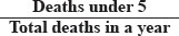
Each disease usually begins with entry of the agent → subclinical phase → mild/moderate/severe clinical phase → recovery, death or disability (organ amputation/prosthetics/carrier states in case of communicable diseases, etc.) (Fig. 1.2). This is usually the spectrum of a disease.
Iceberg of disease
Actually, there are four kinds of people in this world (Fig. 1.3).

Most communicable diseases have an asymptomatic period, during which the person spreads the disease without his/her knowledge. Noncommunicable disease, such as cancers, may have a long latent period before presentation and detection. Screening tests are the rapidly applied tests in apparently healthy individuals of a community to detect cases without symptoms.
Perceptions of disease
Over the ages, our ideas of disease causation has gone a few paradigm shifts.
Supernatural. Although enlightened thoughts were not uncommon in ancient civilisations, the belief that diseases were ‘curses’ from above dominated the middle ages.
Germ theory. This was the first scientific insight into causation of disease. It embodies a one to one relationship between microbes and disease, and especially gained momentum in the 19th century. But it was grossly inadequate because microbes represent only a fraction of disease causation.
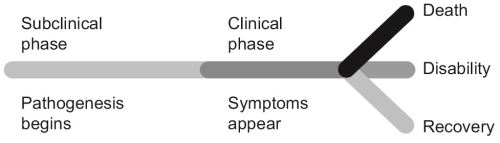
Epidemiological triad. Everyone exposed to a microbe does not get the disease. A tuberculosis Bacilli is particularly prone to infect a malnourished/immunocompromised individual than a healthy one, who live in a filthy environment. This demanded a broader concept of diseases the epidemiological triad of host, agent and environment. Mind the term ‘agent’ here. An agent is any entity that is usually prelude to a disease. It may be a bacterial toxin/cholesterol/carbon monoxide and anything that is the root cause of the disease.
17The multifactorial causation theory. The preacher of multifactorial causation was probably Pettenkofer, but in an age when his words were lost amidst fanatics of germ theory. What he proposed was no less than revolutionary, and has shaped our modern perception of health more than anything. An interaction between various factors ultimately produces a disease often called the risk factors. Relative importance of these factors can be quantified and arranged in order of priority. These factors are only suggestive and not absolute causative agents. Analytical epidemiological studies are used to identify these risk factors.
Web of causes. As the tide of infectious diseases receded, the burden of disease in developed countries shifted to noncommunicable diseases, and we realised that a number of factors operate in collaboration with each other to produce heart disease or diabetes. Not all of them are to be controlled as they have their relative importances. A few important interventions will usually suffice. Example: Male sex and increasing age are nonmodifiable risk factors for ischemic heart disease, but cessation of smoking, exercise and dietary changes offer an affordable protection.
Epidemiologic basis of disease
Consider the statement “Mycobacterium tuberculosis causes tuberculosis”. Hardly surprising. You have been aware of it since your ninth standard. Except that not everyone infected with M. tuberculosis has tuberculosis. Almost everyone of us is infected, but not ill. You’ll insist that the disease affects predominantly people of a certain economic class. So you must rephrase “Mycobacterium tuberculosis causes tuberculosis in lower socioeconomic groups”. And yet its incomplete, because as well as in lower economic classes, tuberculosis is gaining foothold in the middle class, especially those on a tight schedule and health care professionals. Thus you have to rephrase again, and it could go on.
The fallacy is that “M.tb causes tuberculosis” is an epidemiologic truth, which is a concise statement of the epidemiologic triangle of tuberculosis (Fig. 1.4).
Neither one, in isolation, can produce disease.
Natural history of disease/clinical course
The natural history of disease is the evolution of course of a disease overtime uninterrupted by any treatment.
Prepathogenesis. It is the phase before onset of disease but the epidemiological triad is ready. The situation is usually referred to ‘man in midst of disease’.
18Pathogenesis/clinical phase. It is the phase from onset of pathogenesis to termination. It begins with exposure to the agent and the epidemiological triad becomes active. It has two phases—Subclinical (no symptoms) and clinical (symptoms appear).
Physical basis of disease
It is very embarrassing to classify diseases. Most names have been given irrationally by looking at a single sign or symptom (i.e. ‘diabetes mellitus’ meaning ‘frequent sweet urine’) or when more details were known, an underlying pathology (i.e. ‘myocardial infarction’). There is no consistency in the concept of what you call the disease. For example, a man with long standing diabetes mellitus developed hyperlipidemia, which accumulated as an atherosclerotic plaque in his left coronary artery, and culminated in thrombosis of that artery resulting in a myocardial infarction, ending up with left heart failure and pulmonary edema, ultimately the man dying of apnea. So what was his disease?
In this case, his disease should really be called ‘myocardial infarction’, and ‘diabetes mellitus’ an association. The ‘hyperlipidemia’, ‘atherosclerosis’ and ‘thrombosis’ are pathogenic mechanisms in this case, although they may oddly become diseases themselves (it is customary to include anything as ‘disease’ which has some ‘definitive treatment’. Thus hyperlipidemia is a disease but nobody calls ‘hypercreatinemia’ a disease, they simply refer to as ‘renal failure’).
The definitive classification of diseases is published by WHO every 10 years in a book called International Classification of Diseases, Injuries, and Causes of Death. It assigns a three character alphanumeric code to every major condition. Often a fourth character is added for more exact specification: For example, ICD C92 is myeloid leukemia”, which may additionally be specified as C92.0 (“acute”) or C92.1 (“chronic”). Broader groupings are readily formed—For example, ICD C81– C96 consists of all malignant neoplasms of lymphatic and hematopoietic tissue. This system is used for coding death certificates. It determines the presentation of results in the registrar general’s reports and in the diagnostic registers of most hospitals. The system has to be revised periodically to keep pace with medical usage. The ninth revision came into general use in 1979, and has now been superseded by the 10th revision for many applications. The ICD 10 (1993) has a whopping 21 major chapters.
Without delving into such complexity, I have tried to classify diseases from the deepest roots as I can. It will seem odd at first but it is the only way to bring some rationality into it. However, these types are always bound to overlap.
Genetic diseases
Defects in genome may lead to diseases, via enzyme deficiency and altered metabolism. Genetic diseases are on the rise, chiefly due to more exposure to radiation.
Congenital genetic diseases
- Hereditary, i.e. carried over from an ancestor (hemophilia, autoimmune diseases and probably diabetes).
- Mutations—Due to gross mutation during intrauterine life (drug exposure, radiation, congenital anomalies).
- Neoplasia, i.e. ill-regulated growth of tissue due to an acquired mutation in some growth regulating gene.
- Aplasia—The reverse of neoplasia.
Infections
Infections are the major chunk in developing countries. Agents which infect man are viruses, bacteria, protozoan, helminthes, fungi, arthropods and some algae. Infections may cause complications belonging to many other categories in this list.
Diseases of imbalance
Deficiency anemias, malnutrition, vitamin deficiencies, etc. fall in this category. Again, obesity be considered a diseases of excess.
Degenerative diseases
Alzheimer disease, cirrhosis fall into the category of degenerative disease, i.e. replacement of tissue parenchyma by fibers/glia, etc.
Trauma
Accidents and war are man-made epidemics.
Psychiatric diseases
The classification of psychiatric diseases has produced an entire offshoot from ICD, called the Diagnostic and Statistical Manual (DSM).
Risk factors
The gods are just, and of our pleasant vices Make instruments to plague us
—King Lear, V.iii.193 William Shakespeare
An attribute or exposure that is significantly associated with development of a disease. They are only suggestive and not absolute proof of disease occurrence. Also, they must be identified prior to disease occurrence. Risk factors are suspected from descriptive epidemiologic studies and established by analytic studies.
Actually, risk factors represent unclarified ‘agents’—This means the cause effect relationship is usually lacking in them.
Types
- Additive: Smoking + dyes cause additive effect on bladder CA
- Synergistic: Hypertension and hypercholesterolemia potentate each other in development of CHD
- Modifiable: Smoking, hypertension, increased cholesterol in CHD
- Nonmodifiable: Age, sex and genes. This is the risk for which risk groups are mostly defined.
Community risk
Air pollution, water contamination, traffic problem, urban congestion, etc. are risk factors to the health of the entire community.
Risk groups
Presence of risk factors in an individual/group make them more vulnerable to certain diseases. They can be identified by certain definite criteria and more attention is paid to them (risk approach).
Surveillance
It is the
- Ongoing systematic collection, analysis, interpretation of health data
- Essential to planning, implementation and evaluation of public health services
- Closely integrated with the timely dissemination of these data for action.
Simply put – Surveillance is keeping a vigil over the health status of a community and taking necessary steps every moment. It may be said to be the adaptation of health service to changing health status.
Purpose
- To provide information on new/changing trends in health status.
- Timely warning on public health disasters/epidemics.
- Feedback to modify policy or action.
- It helps to plan and set program priority and also to evaluate public health programs (i.e. how good they fare).
Procedure
Collection of data (mainly health indicators) → Consolidation and interpretation of data (i.e. making out information from data – what are the facts behind the figures?) → Dissemination of appropriate plan in demand of changing health status → Action for control and prevention.
Types
- Individual: It is the surveillance of a healthy person/patient while he has a disease or may carry the disease.20
- Local/National/International: Public health problems are kept under close vigil by the nation. Disease like malaria, yellow fever, rabies and relapsing fever are under international surveillance.
- Sentinel: Not all cases report to the government hospitals. Sentinel surveillance aims at identifying missing cases through specialized institutions (like Beleghata ID hospital) or competent individuals (physicians). It is only supplementary to national surveillance but gives more unbiased and detailed data on the cases of a disease and helps find missing cases. A typical example is HIV surveillance which is jointly done by national and sentinel surveillance.
Monitoring
Monitoring may be said to be a small fraction of surveillance. It is the performance and analysis of routine measurements aimed at detecting changes in the environment/21health status of population.Thus we have monitoring on air pollution, growth and nutritional status. In most cases, monitoring is not a medical affair – technicians and instruments can very well measure dust in the air or MAC of a child. To interpret this data (as in surveillance) however, needs professionals.
Three levels of struggle against diseases
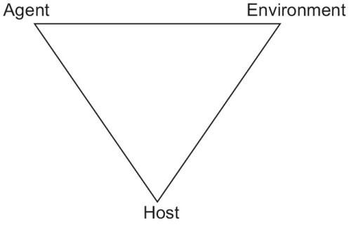
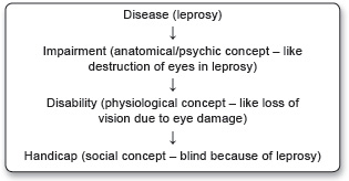
In addition to providing socialized health care to its citizens, the responsibilities of the state also include programs and actions against public health problems—A disease that affects a large number of people, killing/disabling a lot of people and decreasing the productivity of the nation (tuberculosis, malaria, leprosy in India, to name a few). There are three steps, to be followed one after another, to win over a disease (Fig. 1.5; A = agent, H = host, E = environment).
Disease control
The ‘agent’ remains in environment but to such a low level that it ceases to be a public health problem. A state of unstable equilibrium is maintained in the epidemiological triad. It is an ongoing operation and functions by primary and secondary prevention. Its objectives are:
- Reduce number of disease occurrence in community.
- Reduce duration of diseased states.
- Reduce the associated financial burden to the individual and the nation.
Elimination
This means interruption of transmission of disease – by any means. Even after elimination is achieved, apparently, hidden foci of infection may persist and unrecognized methods of transmission may also exist.
The leprosy elimination program was taken up in 1983 and the aim was set at <1 case/10000 population.
Eradication
It means the wiping out of the agent from the environment. It is an absolute goal and have been achieved only for smallpox (May 1980) and Dracunculiasis (2000). Poliomyelitis and measles are serious contenders in line. The criteria for a disease to be eradicated are as follows:
- Should not have an extra human reservoir (in which case that reservoir become a headache, and often the solution becomes to eradicate the reservoir too!).
- Should not have a long carrier state (in the 180 days that require to show up a Hepatitis B infection, you will eventually lose patience to know the results of the postexposure prophylaxis).
- Should have good tools to fight against (AIDS can’t be eradicated until better antiretroviral drugs, and at least a vaccine are in).
- Cases should be easily detectable.
- Should not have subclinical cases (patients who don’t come to doctor make the health status worse and actually help the disease to survive).
- International cooperation is necessary to eradicate a disease.
Prevention
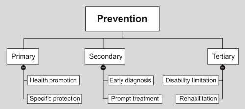
Recall the definition of preventive medicine: Preventive medicine is the art and science of health promotion, disease prevention, disability limitation and rehabilitation (Fig. 1.6).
Primary prevention
These are the activities directed to prevent the occurrence of disease in a human population. The aim is to prevent disease and prolong life.21
Health promotion. “The process of enabling people to increase control over their health and its determinants, and thereby improve their health”.22 Health promotion consists of all the activities which are not aimed at any specific diseases but serve to improve the host factor in epidemiologic triangle.
- Health education.
- Environmental modification (reducing air pollution, safe water, sanitary latrines, control of insects and rodents, improving housing).
- Genetic and marriage counseling (to prevent congenital diseases, i.e. Thalassemia).
- Increasing the standard of living (i.e. the income, education and occupational status).
- Health legislation, i.e. forming rigid standards of health care, sanitation and issues relating to health.
Specific protection. The measures which target particular diseases. The idea of specific protection, especially that killer diseases could be stopped by simple interventions such as ‘vitamin oils’ and ‘shots’ gained mass acceptance in between 1970–1990s.
- Immunization.
- Nutrient supplementation (vitamin A, iodine).
- Chemoprophylaxis (prior medication to at risk population).
- Protection against occupational hazards (masks and sound mufflers for workers).
- Avoiding allergens (for asthmatics).
- Quality control of consumer products (salt—For iodine deficiency diseases, drugs—To avoid adverse drug reactions, cosmetics—To avoid allergy).
Secondary prevention
Those actions which halts the progress of a disease in an individual at the incipient stage and prevents further complications. It is indeed prevention because it prevents further spread of that disease from that individual.
- Early diagnosis
- Screening tests are done in healthy population of a community (i.e. PAP smear).
- Case finding means diagnosing something else in patient other than his chief complaint.
- Special medical examination of risk groups.
- Prompt treatment: A quick cure, helps the patient as well as stops further spread of disease.
Secondary prevention has the disadvantages of being more expensive, less effective in prevention/relief and it fail to prevent loss of productivity to community – as the individual is already diseased.
Tertiary prevention
All measures available to
- Reduce or limit impairment and disabilities
- Minimize suffering caused by existing disease
- Promote the patients adjustments to irremediable conditions.
Tertiary prevention alleviates the pain of the patient who has already been scarred by a disease.
Disability limitation
Disability can be limited by proper treatment – in this case with MDT.
Types of handicap
- Physical—Poliomyelitis
- Mental—Autism
- Social—Orphans.
Rehabilitation:Combined use of:
- Medical, social, educational and vocational measures
- For training and retraining the disabled individual
- To the highest possible level of function.
There are four dimensions of rehabilitation
- Medical: If possible restoration of function (physiotherapy/gadgets, etc.)
- Vocational: Restoration of capacity to earn a livelihood (training and creating jobs)
- Social: Reintroduction into family, kins and society as a whole and involving everyone to maintain the same relationship with this person.
- Psychic: Restoration of self-esteem and confidence.
STATISTICS
There are three kinds of lies: lies, damn lies, and statistics.
—Benjamin Disraeli
The mathematicians dilemma
Science believes in generalizing the special, to make general rules that apply to everybody, from a limited number of observations. This is the only way research is possible, because it is not humanly possible to examine every human on this planet to verify if he has a set of femurs. When Vesalius cut up his very first corpse, he instantly made the decision that the human species, not just the specimen on his table, but the entirety of the human species, must have two femurs. Herein lies the mathematician’s dilemma. A formal proof, as iterated in pure mathematics, should not be based on induction (that is, no one specimen should be held representative of whole of the population). A proof must establish, by mathematical procedures, an identity between two sides of an equation. This kind of reasoning, however smart it may sound, is absurd in most kinds of research except pure mathematics. For the more mundane kind of research, we cannot examine whole populations and we have to deal with samples. A few questions immediately spring up—
- What should be the sample size to make a reasonable conclusion (i.e. can I make a statement “every human has two femurs” by examining only one corpse, or do I need more samples).
- What should be the benchmark of ‘statistical significance’ (i.e. how can I decide if between two events, one is being caused by another, or if its just by chance—There is no real relationship between them).
- What will be the amount of error (how valid will be our research) when we deviate from the mathematical ‘formal proof’ method (i.e. by doing research on samples).
- How much will the research be biased by a distorted sample (i.e. a study done on shoe size on a sample of acromegalics).
Statistics is the answer to these questions.
Data
- Data are the figures you derive directly from the source. Primary data is obtained directly from the population (as in census), and secondary data from a record. Obviously, primary data is always more reliable than secondary.Data has two parts, i.e. a variable (like age, gender, income, number of spouses, etc. denoted by x) and a value (i.e. 40 years, male, Rs. 3500, 3).A variable may be qualitative (Boolean data, subjective data) or quantitative (numbers). Quantitative data may be further classified as continuous (i.e. height, weight which may have any value) or discrete (size of shoes which can have only a fixed set of values).
- Universe is the extent of a statistical survey being undertaken, also called the population. The numerical size of the population is denoted by η. Subgroups in this universe are called samples.
- An event is just that, an event that has or will occur.
Representation of data
The meaning of statistics can ultimately be altered by very easy steps. The simplest is to represent data in such a manner that your boss will find it to easy to comprehend and give you a raise.
Tables
- Simple tables: It is the first thing you have to do with any data. Be sure that everything is readable, the entries have some order (i.e. alphabetical listing) in them, and the table has a title.
- Frequency distribution tables: It describes the frequency of an event within class intervals of a universe. Mind that the class intervals (the domains) do not overlap and are of equal width. A title should unambiguously show what the table contains.
|
Diagrams
There are only a few fundamental types of diagrams.
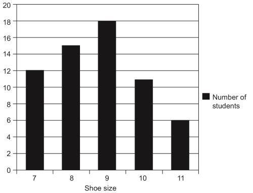
- Bar diagram: Prepare the bars with same width and also same gaps between them.
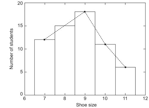
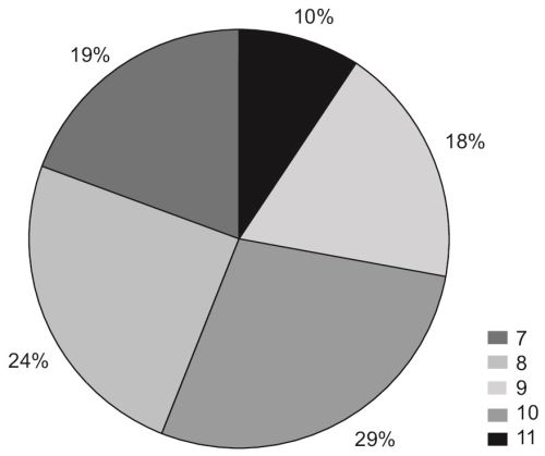
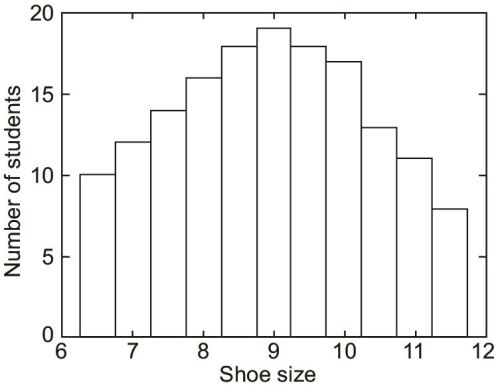
- 27Histogram: It is similar to a bar diagram except that the area of the blocks count. It is the representation of an FD table, so the bars are adjacent (to emphasize the continuous nature of the variable being measured, in this case, shoe size, which can be any value between 7–11). By adding the midpoint of top of these bars – you can get a frequency polygon.
- Pie charts: It represents categories of data as percentage of total and makes a circle of it. Use specific symbols for each category and make a legend outside. Write only the percentages outside the circle.
Measurements
By definition, any set of rules for assigning numbers to attributes of objects is measurement. Not all measurement techniques are equally useful in dealing with the world, however, and it is the function of the scientist to select those that are more useful. The physical and biological scientists generally have well-established, standardized, systems of measurement, unlike social scientists.
The issue of measurements were discussed in great detail by SS Stevens in an article in 1951.
Properties of measurement scales
Magnitude
The property of magnitude exists when an object that has more of the attribute than another object, is given a bigger number by the rule system, i.e. If A is heavier than B then weight of A is more than weight of B.
Intervals
The property of intervals is concerned with the relationship of differences between objects. If a measurement system possesses the property of intervals it means that the unit of measurement means the same thing throughout the scale of numbers. That is, an inch is an inch is an inch, no matter were it falls immediately ahead or a mile down the road.
Rational Zero
A measurement system possesses a rational zero if an object that has none of the attribute in question is assigned the number zero by the system of rules. The object does not need to really exist in the “real world”, as it is somewhat difficult to visualize a “man with no height”. The requirement for a rational zero is this: If objects with none of the attribute did exist would they be given the value zero.
Scale types
In the same article in which he proposed the properties of measurement systems, SS Stevens (1951) proposed four scale types. These scale types were nominal, ordinal, interval, and ratio. Each possessed different properties of measurement systems.
Nominal Scales
Nominal scales are measurement systems that possess none of the three properties discussed earlier. Nominal renaming scales apply random numbers (or words) to objects (i.e. social security numbers, classification of diseases). Nominal categorical scales apply a different number to each category of objects (i.e. Belgians = 1, Indians = 2, Irish = 3).
Ordinal Scales
Ordinal scales are measurement systems that possess the property of magnitude, but not the property of intervals. The property of rational zero is not important if the property of intervals is not satisfied. Anytime ordering, ranking, or rank ordering is involved, the possibility of an ordinal scale should be examined. As with 29a nominal scale, computation of most of the statistics described in the rest of the book is not appropriate when the scale type is ordinal. Rank ordering people in a classroom according to height and assigning the shortest person the number “1”, the next shortest person the number “2”, etc. is an example of an ordinal scale.
Interval Scales
Interval scales are measurement systems that possess the properties of magnitude and intervals, but not the property of rational zero (i.e. the height of a person). It is appropriate to compute the statistics described in the rest of the book when the scale type is interval.
Ratio Scales
Ratio scales are measurement systems that possess all three properties: Magnitude, intervals, and rational zero. The added power of a rational zero allows ratios of numbers to be meaningfully interpreted, i.e. the ratio of John’s height to Mary’s height is 1.32, whereas this is not possible with interval scales.
Sampling
The use of sampling has already been underlined.
Random sampling
Random sampling is left entirely to nature’s own laws of entropy, and everyone has equal probability of being selected. It provides the greatest number of possible samples, but it is also most prone to produce a distorted sample. For example, out of fifty girls and fifty boys, a random sample of 20 has to be chosen. Now it is perfectly possible that the sample of 20 that we choose has exactly 10 girls and 10 boys. It is, however, much more probable for our sample to be distorted either way, i.e. we could select more girls than boys or vice versa. It is, by sheer chance, also possible that we select only girls, and that would be an embarrassingly distorted sample, not even close to representating the population.
Matched random sampling
If we really want to do a scientific study, let’s say about the pattern recognition skill differences between boys and girls, we must select pairs of a boy and a girl, who are identical in all aspects (age, mental growth, family background, etc.) except that one is a boy and other a girl. We could make a comparison only if such matching has been done.
Systematic sampling
Suppose we pick every 10th person from our hundred (i.e. 1, 11, 21, 31 … or 4, 14, 24, etc.), which reduces the number of possible samples (in our particular case, only 10 samples can now be chosen, beginning from 1, 11, 21 to 9, 19, 29). However, if the boys and girls are so arranged that every 10th person is a girl (i.e. if there is periodicity in the population and we resonate with that periodicity), we would end up with 10 girls again. This is the drawback of systematic sampling.
Stratified sampling
We could divide the population into reasonable groups (strata) and then takes samples from each group so that no group gets predilected (we could split our hundred into ‘boys’ stratum and ‘girls’ stratum, and then go on random/systematic sampling within each stratum; this way ensure that we do not end up with only girls or only boys in our sample). Stratification can be done on the basis of age, sex, religion or any other attribute.
Cluster sampling
We could also set up groups of 10 among our hundred (each group may include both boys and girls) and select one from each group. This kind of sampling is used in immunization survey among children.
Errors in sampling
Sampling error
Each sample of a universe differs from another sample, and this is unavoidable, omnipresent whim of nature.
Nonsampling errors
- Overcoverage: Inclusion of data from outside of the population.
- Undercoverage: Sampling frame does not include elements in the population.
- Measurement error: The respondent misunderstand the question.
- Processing error: Mistakes in data coding.
- Nonresponse: People unwilling to take part in a survey may get included in the sample.
Calculation of sample size
Where the sample and population are identical in characteristic, statistical theory yields exact recommendations on sample size (the formulae are, however, not exactly nice looking, and perhaps best to avoid in this textbook). However, where it is not straightforward to define a sample representative of the population, it is more important to understand the cause system of which the population are outcomes and to ensure that all sources of variation are embraced in the sample. Large number of observations are of no value if major sources of variation are neglected in the study.
Patterns of data
Consider the shoe sizes in a class. There will be few short ones, a few large ones, but most of the children will fall in between. Every data observed from nature has two opposing characteristics.
- The tend to accumulate in and about a central figure (central tendency)
- But nevertheless, some of them stand out far from this figure (dispersion).
Measures of central tendency
- The mean is the arithmetic average, denoted by anor μ. It is not, however, a very good indicator of the actual distribution of the variable. Suppose you admit a dinosaur (or any fellow with really big feet) in your class, then the 31mean shoe size will be dramatically altered even though only one member has been added. Mean is affected severly by the values at the end.

- The median is the midline value of a distribution arranged in ascending order, or the average of two midline values (if number of data is even). The median is not affected by terminal values.
- The mode is the most commonly occurring value in a distribution.
Measures of dispersion
Range
It defines the normal limits of a variable. Range of a biologic variable is worked out only after measuring the characteristic in large number of healthy persons of the same age, sex, class, etc. Range gives an idea of how big is the universe, but not anymore about the details.
Mean deviation
A particular value x of a variable is said to be deviating from the mean  by an amount x -
 . This is the deviation of x from mean. The mean deviation is the average of all such deviations.

The mean deviation gives an idea on how widely the data varies. Mind the absolute value sign ‘|’ around the deviations. If we do not ignore the sign of deviations, positive and negative variations tend to cancel each other out. Say the shoe sizes in a class of 11 (in ascending order) are 6,6,7,7,7,8,8,9,9,9,10. The mean, in this case, is ∑x/η = 7.818. Lets calculate the mean deviation.
Student number | Shoe size (x) | Mean (  | Deviation (x -  | |x -  | Mean deviation (|x -  |
|---|---|---|---|---|---|
1 | 6 | -1.818 | 1.818 | ||
2 | 6 | -1.818 | 1.818 | ||
3 | 7 | -0.818 | 0.818 | ||
4 | 7 | -0.818 | 0.818 | ||
5 | 7 | -0.818 | 0.818 | ||
6 | 8 | 7.818 | 0.182 | 0.182 | 12.182/11= 1.107 |
7 | 8 | 0.182 | 0.182 | ||
8 | 9 | 1.182 | 1.182 | ||
9 | 9 | 1.182 | 1.182 | ||
10 | 9 | 1.182 | 1.182 | ||
11 | 10 | 2.182 | 2.182 | ||
86 | 12.182 |
Variance
It is the ∑(x -  )2/η. The variance of a population shows how widely it is distributed. Suppose, in two different classes, the mean shoe size is same. In this 32case, the class with the more variance has a more varying set of students (i.e. there are more number of students who have a very small or very large shoe size) than the class with less variance. Variance is only a number, and its unit is the square of the unit of the thing we want to measure.
Standard deviation
This is important. Standard deviation is the square root of variance.
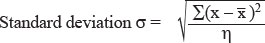
when dealing with the whole universe, or
σ = √[ ∑ (x -  )2 / η-1 ], when in a sample (Bessel’s correction)
Student number | Shoe size (x) | Mean (  | Deviation (x -  | (x -  | Variance ∑ (x -  |
|---|---|---|---|---|---|
1 | 6 | -1.818 | 3.305 | ||
2 | 6 | -1.818 | 3.305 | ||
3 | 7 | -0.818 | 0.669 | ||
4 | 7 | -0.818 | 0.669 | ||
5 | 7 | 86/11 = | -0.818 | 0.669 | |
6 | 8 | 7.818 | 0.182 | 0.033 | 17.635/11= 1.603 |
7 | 8 | 0.182 | 0.033 | ||
8 | 9 | 1.182 | 1.397 | ||
9 | 9 | 1.182 | 1.397 | ||
10 | 9 | 1.182 | 1.397 | ||
11 | 10 | 2.182 | 4.761 | ||
86 | 12.182 | 17.635 | 1.603 |
The standard deviation = √variance = √1.603 = 1.266. After Bessel’s correction, variance = 17.635/(11 – 1) = 1.763 and SD= √1.763 = 1.327.
Properties of standard deviation
For constant c and random variable x,
σ(x + c) = σ(x) (the SD is not changed if each value is incremented by same amount)
σ(cX) = |c| × σ(x) (i.e. if each value of a population gets multiplied, the SD is also multiplied).
Importance of standard deviation
The standard deviation serves as the ‘unit’ of variability. We speak ‘the shoe size of this student is 3 standard deviations (i.e. 3 × 1.266) more than the mean, i.e. the shoe size is mean + 3 × standard deviation = 7.818 + 3 × 1.266 = 11.616.
Probability
As much as we are fond of data and patterns of data, there is always a limit to how much data we can collect, and at some point of time, we have to stop collecting data and do some hypothesizing. It would have been very fortunate if we could 33measure all the data about every aspect of everybody, but until that happens, we have to indulge in speculation and forecasting. The beauty of inferential statistics is that, not only does it allow you to make a reasonable prediction, but also allows you to specify the possible amount of error (i.e. “I am 93% sure that there is 13% chance of rain today”). Probability is a theory of uncertainty which deals with these speculations. It is a necessary concept because the world according to the scientist23 is unknowable in its entirety. However, prediction and decisions are obviously possible. As such, probability theory is a rational means of dealing with an uncertain world.
Probabilities are numbers associated with events that range from zero to one (0–1). A probability of zero means that the event is impossible. For example, if I were to flip a coin, the probability of a leg is zero, due to the fact that a coin may have a head or tail, but not a leg. Given a probability of one, however, the event is certain. For example, if I flip a coin the probability of heads, tails, or an edge is one, because the coin must take one of these possibilities.
In real life, most events have probabilities between these two extremes. For instance, the probability of rain tonight is 0.40; tomorrow night the probability is 0.10. Thus, it can be said that rain is more likely tonight than tomorrow.
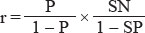
The ‘odds’ of an event. The probability of an event happening/the probability of it not happening. If the probability of rain tonight is 0.3, the odds of rain tonight are 0.3/(1–0.7) or 0.3/0.7.
The meaning of the term probability depends upon one’s philosophical orientation. In the CLASSICAL approach, probabilities refer to the relative frequency of an event, given the experiment was repeated an infinite number of times. For example, the .40 probability of rain tonight means that if the exact conditions of this evening were repeated an infinite number of times, it would rain 40% of the time.
In the SUBJECTIVE approach, however, the term probability refers to a “degree of belief/ confidence.” That is, the individual assigning the number 0.40 to the probability of rain tonight believes that, on a scale from 0–1, the likelihood of rain is 0.40. This leads to a branch of statistics called “Bayesian statistics.” This has lead to the term confidence intervals for the zones in the normal curve (i.e. that a 95% of values lie within 2 standard deviation means that I have confidence that 95 of 100 values will be in this zone).
No matter what theoretical position is taken, all probabilities must conform to certain rules. Some of the rules are concerned with how probabilities combine with one another to form new probabilities.
- For example, when events are independent, that is, one doesn’t effect the other, the probabilities may be multiplied together to find the probability of the joint event.P(A and B) = P(A) × P(B) when A and B are independent eventsThe probability of rain today AND the probability of getting a head when flipping a coin is the product of the two individual probabilities.
- When two events are mutually exclusive, i.e. only one of them is possible at a time, then P(A or B) = P(A) + P(B)
P(A or B or both) = P(A) + P(B) - P(A and B).
Testing for truth
Truth must ultimately be tested. The material sciences (physics, chemistry) usually provide us with the tools to conduct the tests, but it is statistics which tells how to interpret the test. Common to all tests is to find association between two events, i.e.
- To test whether the finding of bronchial sounds is diagnostic of pneumonia (a diagnostic test).
- To test whether smoking is associated with lung cancer (a study to discover risk factors).
- To test whether radiation is effective in lung cancer (a therapeutic test).
All tests must be
- Reproducible, i.e. gives the same result over and over even if different samples are tested, by different observers with different skill levels.
- Accurate, i.e. yields result close to the GOLD STANDARD test, and reflects the true progression of the disease to that level which the test values suggests.
- Valid, i.e. can distinguish between a positive and a negative result (i.e.between diseased and nondiseased) to a satisfactory degree.
Every diagnosis or decision is based on a test, be it the history, a symptom or sign, or some laboratory routines, or the history of an exposure to a risk factor. Such a diagnostic test must bear a few accreditations if it has to qualify for being used in clinical reasoning.
Reproducibility
It is the ability of a test to yield the same results over and over, irrespective of variations in basis of test, method or skill. No test is wholly reproducible. Suppose you have diagnosed a man to have pulmonary tuberculosis by examining sputum smears. A fellow physician may wholly disagree with you, because, when he did the examination, either
- Patient became sputum negative (variation in the basis of the test).
- The physician used a different stain (variation of method).
- The physician made an error in spotting the AFB (variation of skill).
Because no test is wholly reproducible, the whole medical business continues to run on uncertainty.
Accuracy
A test is accurate when
- It yields results equal, on the average, to a GOLD STANDARD test.
- The test result indicates the true progression of the disease.
Suppose you devise method X to determine blood glucose. To qualify as accurate, this test has to yield results consistent with that of the Glucose oxidase reaction; in addition, it must truly reflect the progression of diabetes mellitus.
Validity
This is the challenge: To distinguish truth from just another chance finding.
Put simply, let’s say you attend some kids with complaint of cough, fever and mild dyspnea. You did some auscultation (the test) and find bronchial sounds in some of these kids, and label them as pneumonia. Next, your boss carries out a culture on their lung aspirate (the Gold Standard Test) and disproves your findings. The final scenario is this.
Diseased Culture +ve | Nondiseased Culture –ve | |
+ve test Bronchial sounds | a | b |
-ve test No sound | c | d |
The sensitivity of the test is the probability of diseased people yielding positive result,= a/a+c. The specificity is the reverse, the probability of healthy people to give negative result = d/b+d.
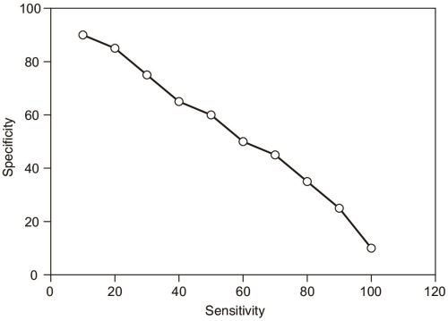
A test which is very nonspecific will yield too many false-positive results; on the other hand, an insensitive test gives too many false-negative results. The importance we attach to a positive or negative result is thus a function of the cut off value of the test, i.e. after which level we consider the results positive. Selecting a low cut off reduces the specificity of the test, and a high cut off dampens sensitivity.24 In fact, the curve of sensitivity vs specificity looks like this (Fig. 1.10).
The perils of using nonqualified tests are many. Too many false +ve results are a burden on the health infrastructure, cause useless anxiety to the victim, and once labeled – it’s hard to get rid of the ‘feeling’ of the disease (consider what goes 36though anyone after being diagnosed HIV +ve). Again, too many false –ve results fail the entire purpose of clinical medicine and screening.
Predictive value
This is the most important aspect of a test from a clinical viewpoint. A positive predictive value is the probability of someone testing positive actually having the disease, i.e. a/(a + b). Similarly, a negative predictive value is the probability of not having the disease in someone testing negative = d/(c + d).
The positive predictive value is affected by the
- Prevalence of the disease—In areas of high prevalence of some disease, tests for the disease are more valid.
- Specificity of the test.
The usual challenge: Determine posttest probability from pretest knowledge
Bayesian statistics states that the positive predictive value is much higher if the disease in question is very prevalent. In another words, the usefulness of a test, apart from an inherent quality of itself (the sensitivity and specificity), is also dependant upon how common the disease is. Suppose the prevalence of a disease in a certain area is P in a population of η; this means, the chance of any individual of that area of having the disease is P (the pretest probability). Now we do the test and get a positive result. Given the specificity and sensitivity of the test, what is the probability that the individual is truly diseased?
Diseased | Nondiseased | Total | |
+ve test | a | b | a + b |
-ve test | c | d | c + d |
Total | a + c | b + d |
Now, obviously, the number of total diseased people a + c = Pη and nondiseased people b + d = (1 - P)η. Again, the positive predictive value is (number of diseased people who tested +ve/total number of people who tested +ve) = a/a + b.
Given the sensitivity of the test is SN and specificity is SP, we know that

From these equations, calculate your heart out for the value of positive preditive value a/a+b; you will find it to be
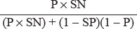
This is the positive predictive value of a test if the sensitivity, specificity and prevalence is given. There is, however, a more subtle way to achieve the same result. The odds of an individual having the disease before the test is, obviously, P/1 – P (see definition of Odds). Now, Bayesian statistics states that the odds (r) of having the disease after a positive test is

This x is the posttest probability or the positive preditive value (do the actual calculation on a real problem and you will find the result from the two methods to be identical). The factor sensitivity/1-specificity is called the likelihood ratio of the test.
Hypothesis testing
I mentioned earlier that inferential statistics allows you to predict both the probability of an event and the amount of error of that prediction. This section is to determine that amount of error.
The usual hypotheses
The null hypothesis (H0). It states that there is no relation between the two events tested.
The alternate hypothesis (Ha). It states that the two events are related.
Obviously, both cannot be true simultaneously.
Errors
Type I error (α). The error that happens when null hypothesis is rejected in spite of it being true (i.e. you wrongly diagnose an association between traveling to Goa and ulcerative colitis, or something equally bizzare). The probability of a Type I error happening in a test is called p value or α limit of the test.
Type II error (β). The error that happens when the null hypothesis is accepted in spite of it being false (you miss a true association)
The power of a test, i.e. the probability that a test detects any difference that actually exist, is 1 - β.
Tests for statistical significance (Fig. 1.11)
The normal distribution
The idea of the normal distribution is primary to hypothesis testing. In collecting data, if our sample is large enough, we tend to have a distribution much like that of our shoe size example (Fig. 1.12).38
When we connect the top of the bars, we get a curve like this (Fig. 1.13).
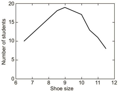
If we plot the y-axis from 6 instead of 0, as to emphasise the variations, not actual values, then we get (Fig. 1.14).
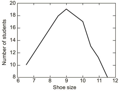
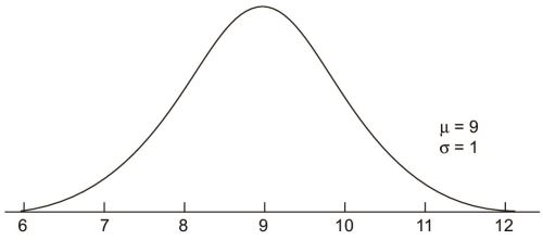
39If we could go on, and collect show size data of an infinite number of students, and if shoe sizes would vary continuously (that is, the class intervals, would be adjacent—There was no discrete jumps from size 6 to 6.5 but 6.1, 6.11 and so on), we would actually produce a normal curve. It is a curve which has been sketched after infinite number of observations and with no gaps in between class intervals. Because the curve is absolutely hypothetical, it is a bell-shaped, symmetrical curve with absolute continuity (Fig. 1.15).
The standard normal curve
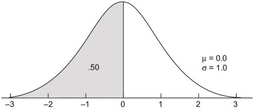
The standard normal curve is a member of the family of normal curves with μ = 0.0 and σ = 1.0. The value of 0.0 was selected because the normal curve is symmetrical around μ and the number system is symmetrical around 0.0. The value of 1.0 for σ is simply a unit value. The x-axis on a standard normal curve is often relabeled with multiples of σ and called z-scores.
There are three areas on a standard normal curve that all introductory statistics students should know. The first is that the total area below 0.0 is .50, as the standard normal curve is symmetrical like all normal curves. This result generalizes to all normal curves in that the total area below the value of μ is .50 on any member of the family of normal curves.
The second area that should be memorized is between z-scores of -1.00 and +1.00. It is .68 or 68%.40
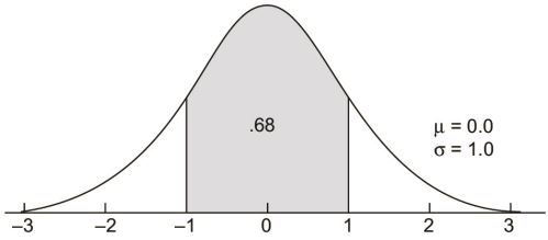
The total area between plus and minus one sigma unit on any member of the family of normal curves is also .68.
The third area is between z-scores of -2.00 and +2.00 and is .95 or 95%.

This area (.95) also generalizes to plus and minus two sigma units on any normal curve.
Conversion of a normal curve to a standard normal curve
Suppose a variable x has a mean  and a standard deviation σ. It will produce a normal curve, no doubt. But it is easier, if we want to emphasize the variation rather than the actual values, to plot it in a standard normal curve by making the mean 0 and standard deviation 1 (Fig. 1.16).
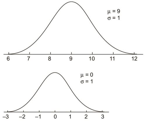

Now plot the curve of z. The curve of z is shifted parallel to x and is reduced in size, but the fractional areas under confidence intervals remain the same.
Skewed distributions (Fig. 1.17)
- Positively skewed—Mode < median < mean
- Negatively skewed—Mode > median > mean
Remember that mean is always dragged towards the tail of the distribution.
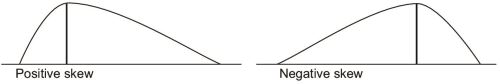
Probability and the normal curve
Each particular area bound between any two z-scores (any two vertical lines over the x-axis) is associated with a certain degree of probability, and all such areas are called confidence intervals. In continuum with our example of shoe sizes, what of those students who have a size of 11.5 or more? Could they be considered acromegalics, or perfectly ‘normal’ people? Look at the normal curve of shoe sizes again, the size 11.5 lies outside two standard deviations (11 in our curve). The area inside two standard deviations in a normal curve, as I have already illustrated, is 0.95. Thus the area outside 2 standard deviations is obviously, 0.05. This means that the person with a shoe size of 11.5 has a 0.05 probability (or 5%) chance of being normal.
Levels of significance and p-values
We have mentioned that 95% of values lie within 2 standard deviations around the mean. This means, 5% of values lie outside (thus called ‘outliers’). This is called the alpha limit of two standard deviation. A p-value or probability value can be calculated for each interval in the normal curve (recall that the p-value is the probability of a Type I error, i.e. a false association is diagnosed). The p-value indicates the probability of a member from that interval being selected in a random sample. A p-value outside this limit ( < 0.05) is statistically significant, i.e. if the members of this interval (the last 5% area under the normal curve) appear in a random sample, that sample has 5% chance of being representative of the population. Similarly, p-value may be deduced for any confidence interval.
Binomial distribution
Not every variable (in fact, none) is distributed normally. For the real world with its variations, inequalities and heterogeneities, statisticians have found certain patterns of how certain events tend to happen. These ‘models’ of reality are known as ‘statistical distributions’.
42Let’s say that a certain event has only two outcomes, such as tossing a coin. It has two possible outcomes head (H) and tail (T). Let p be the probability of head, q be the probability of tails. Clearly, from an abstract, neutral viewpoint, both p and q equal 0.5.
Now we do the tossing twice. The possible number of outcomes now become four (HH, HT, TH, TT). What is the probability of each of these occurrences? Remember that the probabilities of two independent events get multiplied if that are to occur together. The outcomes of the two tosses are independent (i.e. the results of the first toss does, in no way, affect the second), so probabilities must be multiplied.
Outcome | Probability |
HH | p × p = p2 |
HT | p × q = pq |
TH | q × p = pq |
TT | q × q = q2 |
The total of all probabilities, i.e. summation of all possible outcomes of a binary event (as in a coin toss), is the binomial distribution. When tossing only twice (n=2), the summation is p2 + 2pq + q2. For tossing n times, we can generalize the formula by mathematical induction

which results in the expansion (following Newton’s binomial theorem; nCr denotes possible combinations of r things among n slots)

or, to put it concisely (review the formula of combinations from your class XII algebra book)
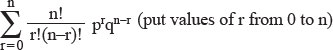
where r is number of times we get a ‘head’ out of those n number of tosses, and we denote a ‘head’ as our success. Now let’s put Aside all this coin business and do some real research. Suppose Aspirin cures, and has been curing, most headaches (80% of the times) since time immemorial. Now you introduce a new drug ‘headgone’ that boasts 98 cures out of 100 patients who have tried it. Is it really any significant improvement over Aspirin?
Apart from the pharmacological issues (its pharmacokinetics and safety profile), let us be purely statisticial. The time tested Aspirin cures headaches 80% of the time, so that probability of cure by aspirin p is 0.8; obviously, probability of no relief with Aspirin q is 0.2. With the new drug, we have had 100 patients and tried our luck to see whether they are relieved. Its exactly the same as tossing a coin (the new drug) 100 times (on 100 patients) and assesing cure or no cure (just like heads or tails). 98 of them were cured, so our ‘success’ r is 98. If we assume the null hypothesis H0 is true, then it follows that this new drug is no different from 43Aspirin, and the number of times it cures is no different from Aspirin. So we can, in effect, apply the results of this drug to Aspirin and see what is the probability that Aspirin will cure 98 out of 100. We choose, from the many terms in the binomial expansion of (p + q)n (see earlier), that particular term which matches our particular r which is 98.
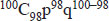
which equals to

What this means is that the probability of 98 out of 100 cures by Aspirin is so low that it cannot be even be expressed properly in decimals (and we have to resort to scientific notation), but this new drug has already done it. So we conclude that ‘headgone’ must actually be better.
Student’s26 test and the t distribution
Suppose in the mean of a population (or universe, as we’ll call it) is μ. Each sample from this population has a different mean ( ) value. These means, if plotted are found to be normally distributed around the universal mean μ. If we take any number of samples (each containing n members27), then each sample will have its own mean
  . It is perfectly possible that we choose a sample from the lower end of the universe, i.e. only the shoe sizes between 6–8, so that we get a sample mean = 7. It is also possible that we get, in our sample, only the largest shoe sizes, giving a sample mean = 11. But if we go on taking random samples, chances are that we would encounter every shoe size in most of our samples. So the means of our samples could be any or all of 6, 6.5, 8, 8.5, 11.5 or any plausible value. If we go on taking infinite number of samples, we would, obviously, get an infinite number of sample means. The mean of these infinite number of means, as we will find out, will be equal or very close to the universal mean μ, and the sample means themselves will form a normal curve. This ‘normal curve of the sample means’ will, again, have the universal mean μ as its mean. This is the central limit theorem.

Figure 1.18: Normal curves of small samples taken from the population shown along with the universal curve
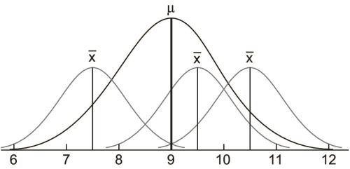
44The same rules of normal curve apply these sample means also, i.e. if a sample has a mean outside, say 2 standard deviation about the universal mean  , it has little (5%) chance of being selected (i.e. it is not a representative sample of the population).
The standard deviation of these sample means is called the standard error of the mean. This is equal to, as you see, SD of the original distribution/root of number of members in the sample (σ/√n). Thus there is also a relative deviate of these sample means (analogous to the z-score of a normal curve), which we denote by t.
t = (Mean of a particular sample—Mean of all sample means)/Standard error of the mean = 
To determine whether a sample is representative, we need to know
- The t-value of the sample.
- The degree of freedom, which is one less than the number of members in the sample (n - 1).
- Standard t distribution table.
For examples, lets say that the mean (μ) of shoe sizes in the entire class (universe) is 9, and standard deviation (σ) is 1. We take a sample of 21 (n) students and measure their shoe size, and the mean of this sample ( ) is 10.12. Now, the t-value of this sample is = ( - μ)/(σ/√n) = (10.12 – 9)/(1/√20) = (1.12) / (1/4.472) = 5.006
|
Find the t-value corresponding to the degree of freedom in this table, which matches less than or equal to the value in our result (i.e. 5.7). That particular t-value in this table is 2.79, which indicates a p-value of < 0.05 (see the top row of the table). Thus, the difference of shoe size in this particular sample from the average of the class is statistically significant.
Note that in this case, we take the whole population (universe) to compare with our sample. But the test could well be used to compare two samples, and the universe itself could serve as a sample. In fact, the unpaired t-test is most useful for comparing two samples. A second kind of t-test, the paired t-test, is useful for comparison of the same sample before and after an intervention.
The paired t-test
Suppose the mean shoe size in a class of 30 is 9.5. For a month, we apply growth hormone injections in each of the students and then measure their shoe sizes again. 45This time, we find the mean show size to be 10.3. Does this indicate a statistical difference?
Like all statistical tests, we assume that there is, actually, no differences and the children grew up due to their natural growth spurt, not our hormone injections. To test this hypothesis, we must find the difference in shoe size of each individual student before and after injection, which we call d. Obviously, for 30 students, we will get 30 differences (d1, d2, d3 ... d30). The summation of these differences (∑d) divided by number of students (η) in this case 30, is the average difference or d. The null hypothesis, states that the value of d¯ (i.e. there should no difference).
Now comes a crucial step. If these differences (d1, d2 are plotted, they will form a distribution among themselves. Some students will have grown much more than others (high difference) and some not much (low difference). We could, in theory, deduce of standard deviation of differences, which is
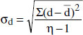
The t-value, in the paired t-test is

This t-value is checked, in the standard t table, for a degree of freedom η - 1, and a p-value could be deduced. Note the central theme in paired t testing is that we use the mean and standard error of differences before and after intervention, rather than using actual values.
The unpaired (independent) t-test
While comparing the shoe sizes of two classes, we assume that there is no difference in shoe sizes at all between the two classes (the null hypothesis). Because the two classes are nor paired (the same student cannot read in two classes) neither are the number of students the same in two classes, we cannot measure the standard deviation of differences directly, as we did in the paired t-test. Thus find the pooled standard deviation of two classes, which is

where η1, η2 are the number of students in two classes, respectively, and σ1 and σ2 are the standard deviations of shoe sizes in those classes. The t-value, in the unpaired t test, is
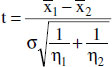
χ2 test
It is the test applied where two groups of subjects, with differing characteristics, have to be tested for a common variable. They are first arranged in Table 1.7.46
|
We assume that shoe size is no indicator of acromegaly (the null hypothesis). Then the ones with small shoes are expected to have the same rate of acromegaly as those with large shoes (and that should be the prevalence of acromegaly in whole population in general). The incidence of acromegaly in whole population is a+c/(a + b + c + d). Thus expected numbers in the four cells are calculated likewise, i.e. expected number in cell ‘a’ is total number of students with shoe size > 11 × incidence of acromegaly in whole population = (a + b) × (a + c)/(a + b + c + d). Similarly, expected number in cell b = Total number of students with shoe size < 11 × incidence of ‘no acromegaly’ (normal children) in community = (c + d)×(b + d)/(a + b + c + d).
χ2 for each cell = (observed number - expected number)2/expected number.
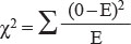
The summation of values of χ2 is calculated. Now the degree of freedom of a table is (rows-1)(columns-1). The probability that matches the χ2 value we just got and the degree of freedom in the χ2 table, if less than 0.05, rejects the null hypothesis.
|
Analysis of variance and the F test
Similar to the t-test, the F test or ANOVA compares three or more samples. It is most useful when three or more groups have variable characteristics (like children with blood groups A, B, AB and O) and need to be compared over a common variable (whether blood group affects shoe size).
Pearson’s correlation
The correlation coefficient is the degree of association between two variables, i.e. if number of observations is n,
A positive r indicated that y increases with x, and the more nearer r becomes to 1, the relationship becomes almost linear. For example, suppose we measure 47the shoe sizes and height of the students in a class and get the following graph (Fig. 1.20).
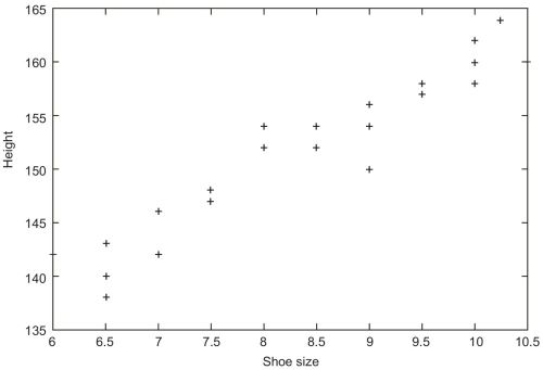
Obviously, this indicates positive correlation (positive r) between shoe size and height. It is possible, if enough data is available, to predict the height from the shoe size of a student, a process known as simplelinear regression. The regression coefficient b is the amount of change of y per unit change of x (δy/δx) which can be calculated from the correlation coefficient r

The value of y for a certain x then becomes a matter of equation

where a is the value of y when x = 0 (the intercept of the correlation line on the y-axis).
Spearman’s rank correlation
If data is not measurable in an interval scale (as we are used to) but in an ordinal scale (‘1st boy’,‘2nd boy’ or ‘Grade I cancer’,’ Grade II cancer’, etc.), then the degree of correlation between two such variables (i.e. ranking of boys in a class and ranking of the same boys in annual sports—as to see whether boys good in studies are also good in athletes) is measured by Spearman’s rank correlation coefficient ρ.
Poisson distribution
The Poisson distribution describes events that are very unlikely, or very random (like rate of disintegration of radioactive atoms). There are many other kinds of distributions, and more details of each, which are more appropriate in a textbook of statistics rather than this one.